Meep Example 14 · 박막 속 점광원, 공기로 나오는 몫 — 광추출 효율, LDOS 정규화, kz 적분, CYL 대 3D
TL;DR (English)
- What: post 11 measured how much a dipole emits (LDOS); post 13 split a body of revolution into m runs. An LED asks for the ratio: of everything a dipole in the emitting layer puts out, how much reaches the air. Extraction efficiency = flux through an open surface in air ÷ the source’s own work from
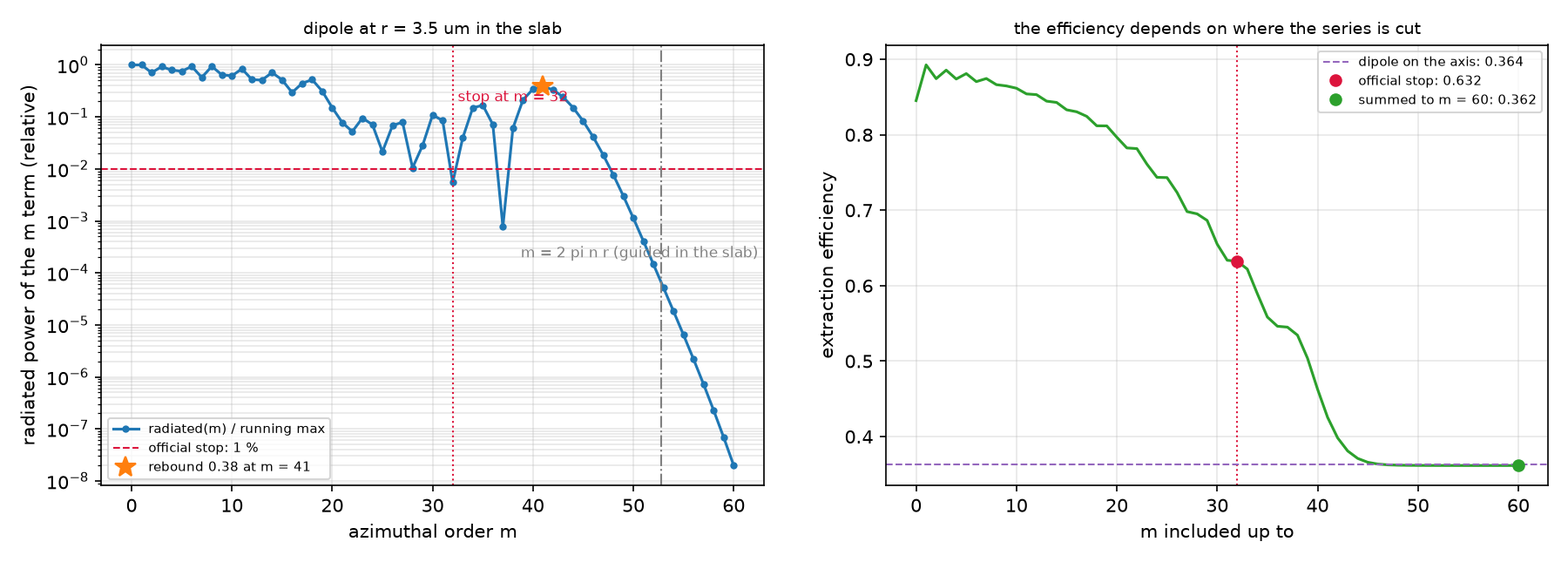
dft_ldos. Three official examples: a dipole in a layer on a mirror (cylindrical vs 3D), the same slab with the dipole off the axis (an m series), and a dipole inside the cleaved facet of a laser stack (a 2D cross-section plus a kz integral). - Result: A dipole halfway up the layer sends 0.323 of its power into air (cylindrical, resolution 80); the efficiency swings from 0.52 near the mirror to 0.09 near the top, and at resolution 40 cylindrical and 3D disagree by up to 16 %: a 0.29 µm layer needs resolution 80. 3.5 µm off the axis, the official stop rule (first m below 1 %) halts at m = 32 and reports 0.632; the series rebounds at m ≈ 41, where the slab-guided emission lives, and the sum to m = 60 gives 0.362, matching the on-axis 0.364. The cleaved laser facet needs 76 kz runs and extracts 22.4 %; a single 2D run (kz = 0) would claim 32.9 %.
- Takeaway: the denominator is not a vacuum constant but the dipole’s own work, and its voxel volume differs between coordinate systems (2πr/res² vs 1/res³ vs 1/res²). Most of the light stays guided in a high-index film. Where you cut a series (m or kz) changes the answer, and the official “first term below 1 %” rule can stop before the guided light arrives.
- Code: full script at the bottom, ~77 min (mpirun -np 4; B alone 58 min).
0. 이 글에서 배우는 것
- 광추출 효율의 정의: 분자는 공기 쪽 열린 flux 면, 분모는
dft_ldos의 source 일 $-\mathrm{Re}(FJ^*)\,\Delta V$ - 좌표계마다 다른 $\Delta V$: cylindrical $2\pi r/\mathrm{res}^2$, 3D $1/\mathrm{res}^3$, 2D $1/\mathrm{res}^2$
- 같은 문제를 cylindrical과 3D로 풀어 맞추는 교차검증. 어디서 어긋나는가
- 축에서 떨어진 쌍극자의 m 급수에서 “언제 멈출까”가 결과를 바꾸는 경우
- 한 방향으로 균일한 구조(절단면 레이저)의 3D 문제 = 2D 단면 + kz 적분
전제 지식: 11편의 dft_ldos, 13편의 cylindrical 좌표와 m 급수. 공식 예제: LDOS 튜토리얼의 LED 추출 효율 · nonaxisymmetric dipole sources · 스크립트 extraction_eff_ldos.py · point_dipole_cyl.py · edge_emitter_2D.py. 이전 글: 13 · 회전 대칭으로 3D를 계산하기 · 다음 글: 15 · 점광원이 수천 개일 때
1. 무엇을 알고 싶은가
13편 끝 질문이었다. 디스크 안의 쌍극자를 LED의 발광층으로 보면, 쌍극자가 낸 빛 중 몇 %가 공기로 나오는가. 굴절률 2.4인 층에서 공기로 나가려면 임계각 25° 안쪽으로 계면에 닿아야 하고, 나머지는 전반사로 층 안을 따라간다. 이 몫을 재려면 두 숫자가 필요하다. 공기로 나간 power와 쌍극자가 낸 전체 power. 앞의 것은 flux monitor로 잰다. 뒤의 것은 11편처럼 거울과 층이 방출량 자체를 바꾸므로 진공의 상수로 둘 수 없고, 그 구조 속에서 source가 한 일로 재야 한다. 그리고 3D 문제를 싸게 푸는 세 길(cylindrical, 대칭을 쓴 3D, 2D + kz)이 같은 답을 주는지 본다.
어디에 쓰이는가
광추출 효율은 발광 소자의 외부 양자 효율(EQE) = 내부 양자 효율 × 추출 효율에서 뒤쪽 인자다. 소자 설계의 대부분이 이 숫자를 올리는 일이다.
| 응용 | 이 글의 어떤 것을 쓰는가 | 그 다음에 필요한 것 |
|---|---|---|
| OLED·LED·micro-LED 발광층 설계 | 높이(전극과의 거리)에 따른 추출 효율, LDOS 분모 | 15편 수천 개의 발광체 |
| 반도체 레이저·SOA의 절단면 | 2D 단면 + kz 적분, 편광별 추출 | 18편 계면의 각도 응답 |
| 양자점·단일광자원 수집 효율 | 축 위/축 밖 쌍극자의 차이, m 급수 | 16편 far field로 모으기 |
| 광추출 구조(텍스처, 렌즈, 광결정) 최적화 | 분자·분모 정의와 교차검증 절차 | 35편 near2far 역설계 |
2. 물리 한 페이지
추출 효율은 두 power의 비다. 분자는 공기 쪽에 둔 열린 flux 면으로 잰다. 분모는 source 점에서 field가 전류에 한 일이고, dft_ldos가 저장한 $F$(field)와 $J$(전류)로 계산한다. source 하나가 차지하는 부피 $\Delta V$가 좌표계마다 다르다.
축에서 떨어진 쌍극자(cylindrical)와 한 방향으로 균일한 구조의 점광원(2D)은 둘 다 급수로 푼다. 앞은 m에 대해, 뒤는 kz에 대해. 서로 다른 m(또는 kz)은 직교하므로 power는 항별로 더한다. ±m과 ±kz는 같은 power를 주므로 0이 아닌 항은 두 배로 센다.
\[\eta_{\mathrm{off\text{-}axis}}=\frac{\sum_m w_m P^{(m)}_{\mathrm{air}}}{\sum_m w_m P^{(m)}_{\mathrm{total}}},\qquad \eta_{\mathrm{edge}}=\frac{P_{\mathrm{air}}(0)+2\sum_{k_z>0}P_{\mathrm{air}}(k_z)}{P_{\mathrm{tot}}(0)+2\sum_{k_z>0}P_{\mathrm{tot}}(k_z)},\qquad w_0=1,\ w_{m>0}=2\]고굴절률 층에 갇힌 빛(guided mode)은 층을 따라 반지름 방향으로 간다. 축에서 r만큼 떨어진 쌍극자가 낸 guided 빛은 방위 차수 $m\approx 2\pi n_{\mathrm{eff}} r/\lambda$ 근처의 항에 실린다. 이 빛이 셀 끝의 옆면 monitor를 지나가면 분자에 들어가므로, 그 m까지 가기 전에 급수를 끊으면 다른 숫자가 나온다.
| 기호 | 뜻 | 코드 변수 |
|---|---|---|
| $\eta$ | 추출 효율 | p_air / p_tot |
| $h$ | 거울에서 쌍극자까지 높이 / 층 두께 | HEIGHTS |
| $F, J$ | dft_ldos가 저장한 source 점의 field와 전류 |
sim.ldos_Fdata, sim.ldos_Jdata |
| $\Delta V$ | source 한 개의 부피 | 2*pi*r/res**2, 1/res**3, 1/res**2 |
| $m$, $k_z$ | 급수의 항 | m=, k_point=(0,0,kz) |
가정과 유효 범위: 파장 1 µm, 손실 없는 층과 완전도체 거울(A·B), 손실 없는 다층(C). 분자는 열린 면이라 “공기 쪽으로 나간 몫”이지 닫힌 에너지 수지가 아니다. 셀의 가로 크기 L(A: 6 µm, B: 20 µm)이 유한하므로 그 밖으로 가는 빛은 옆면에서 센다.
결과 보기 전에 맞춰보기
| 물리량 | 내 예측 | 근거 |
|---|---|---|
| 추출 효율(A, h = 0.5) | 0.3 근처 | 노트 0.323(CYL)·0.337(3D) |
| 높이 의존 | 거울에서 멀수록 변한다 | 쌍극자와 image의 간섭(10편) |
| CYL res 40 vs 80 | 1% 안 | 파장당 40칸 이상 |
| 3D vs CYL | 2% 안 | 노트 max 0.017 |
| 축 위 쌍극자(B) | 0.3 근처 | 같은 층, 다른 셀 크기 |
| B: 공식 종료 규칙 | sum-to-60과 다르다 | 노트: 0.63–0.74 vs 0.36 |
| C: 필요한 kz 수 | 70~80 | 노트 76 |
| C: 추출 효율 | 22% 근처 | 노트 22.4% |
판정 기준: 효율이 0 아래나 1 위면 분모의 $\Delta V$나 flux 면의 부호가 틀렸다. CYL과 3D가 2배 다르면 voxel 부피, 5~10%면 해상도나 source 위치를 의심한다.
3. 시뮬레이션 설계도
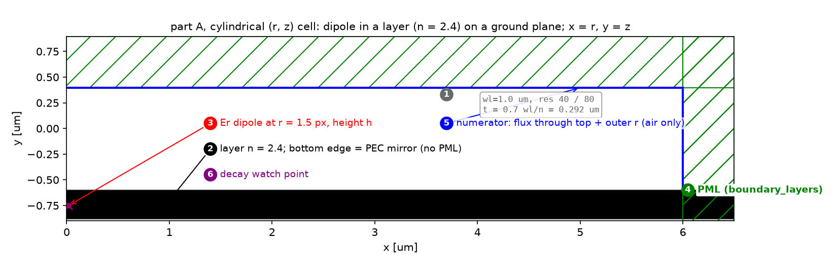 파트 A의 cylindrical (r, z) 셀(x가 r, y가 z). 회색 층이 n 2.4(두께 0.292 µm), 그 아래 셀 벽이 PML 없는 완전도체 거울이다. 빨간 점이 축에서 1.5 픽셀 떨어진 Er 쌍극자, 파란 선이 분자를 재는 열린 flux 면(위와 옆). 파란 빗금은 대표 DFT 영역. 동그라미 숫자는 §4의 단계 번호다.
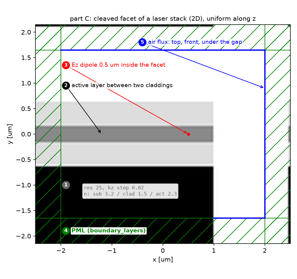 파트 C의 2D 단면. 왼쪽에서부터 기판(n 3.2), 클래딩(1.5), 활성층(2.3), 클래딩이 쌓인 다층이 x = 1.5 µm에서 잘려 있고(절단면), 그 오른쪽은 공기다. 쌍극자는 절단면 0.5 µm 안쪽의 활성층. z 방향으로 구조가 균일하므로 kz마다 2D run 하나를 돌린다.
| 파라미터 | 값 | 왜 이 값인가 | 바꾸면 |
|---|---|---|---|
| A 층 | n 2.4, 두께 0.7λ/n = 0.292 µm, 거울 위 | 공식 값 | 두께가 바뀌면 guided mode 수가 바뀐다 |
| A 높이 | 0.1~0.9, 9점 | 공식 21점의 축소 | — |
| A 해상도 | CYL 40·80, 3D 40 | 공식 80. 3D는 비용 때문에 40 | 3D res 80은 셀 하나 4500만 칸 |
| A 수집면 | 가로 6 µm, 공기층 1 µm | 공식 값 | 좁으면 옆으로 나간 빛을 놓친다 |
| B 셀 | r 20 µm, 층 같음, res 50 | 공식 point_dipole_cyl.py | — |
| B 쌍극자 | r = 3.5 µm, m = 0…60 | 공식 r 중 하나, $2\pi n r\approx53$을 넘게 | 공식은 첫 1% 아래에서 멈춤 |
| C 다층 | 3.2 / 1.5 / 2.3 / 1.5, res 25 | 공식 edge_emitter_2D.py | — |
| C kz | 0.02 간격, 전체 power가 최대의 2% 아래일 때까지 | 공식 값 | 간격이 넓으면 guided 봉우리를 놓친다 |
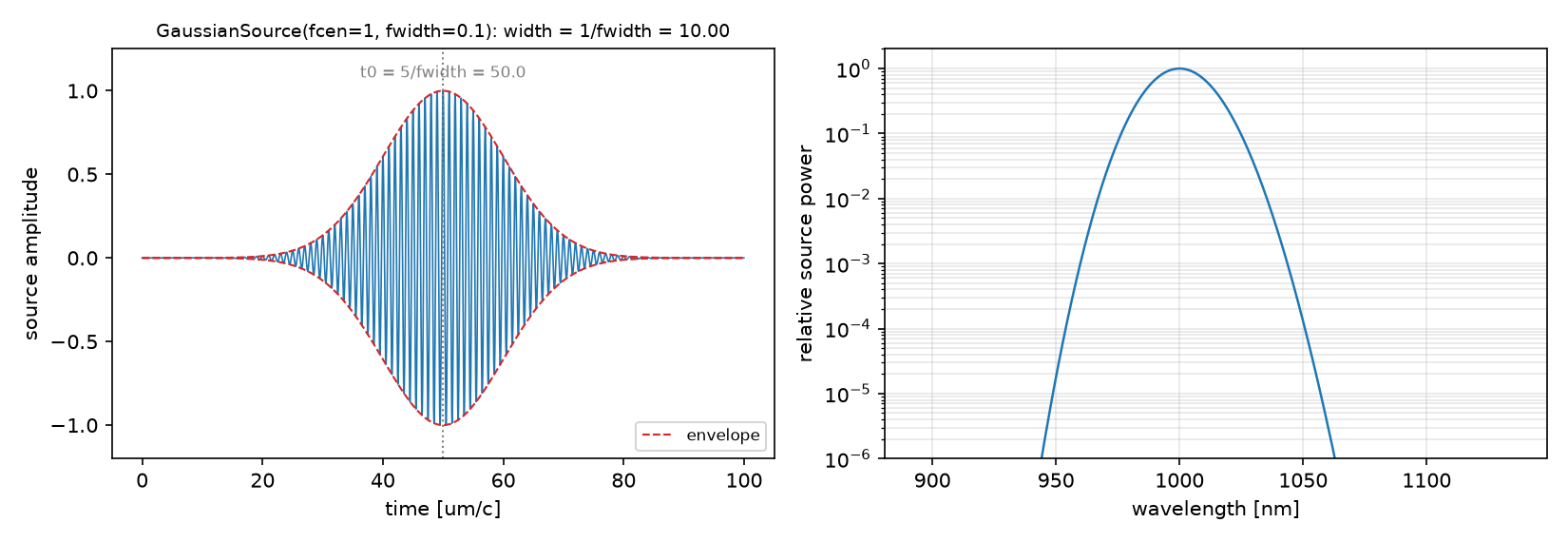 source 파형과 스펙트럼(1000 nm, fwidth 0.1 fcen. B는 0.05). 효율은 중심 주파수 하나에서 잰다.
강의 노트북과의 차이: 강의 범위 밖이다. 10_sources의 세 노트는 각각 공식 조건 전체(21 높이 × 2 좌표계 res 80, r 네 개 × m 수백, kz 76점)를 돌렸다. 이 글은 A의 3D를 세 높이·res 40으로 줄이고, B는 r 하나에서 공식 종료 규칙과 m = 60까지 합한 값을 같은 그림에 놓는다.
4. 코드 따라가기
읽는 순서: 단위·파라미터 → 재료·구조 → source → Simulation·경계 → monitor → 실행·종료 → 후처리. 이번 글의 핵심은 ⑦의 분모다.
① 단위와 파라미터 — 어떤 숫자를 고정하는가
WL, FREQ, N_L = 1.0, 1.0, 2.4
T_L = 0.7 * WL / N_L                      # layer thickness
DPML, DAIR, L = 0.5, 1.0, 6.0             # PML, air above the layer, lateral size of the collection surface
HEIGHTS = np.round(np.linspace(0.1, 0.9, 9), 3)      # dipole height above the ground plane, fraction of T_L
DKZ, KZ_TOL = 0.02, 0.02                  # part C: kz step and stop when the total power falls below 2 % of its max
- 무엇: 층과 수집면, 높이 sweep, kz 간격.
- 왜: 층 두께 0.7λ/n은 guided mode가 하나 남짓 들어가는 두께다. 높이를 바꾸면 쌍극자와 거울 image의 간섭이 바뀌어 방출 방향과 양이 둘 다 변한다.
- 틀리면: 수집면 L이 좁으면 옆으로 비스듬히 나간 빛이 PML로 가 버려 분자가 작아진다.
② 재료와 구조 — 층 하나와 거울
mp.Block(material=mp.Medium(index=N_L), center=mp.Vector3(0, 0, -0.5 * sz + 0.5 * T_L), size=mp.Vector3(mp.inf, mp.inf, T_L))
boundary_layers=[mp.PML(DPML, direction=mp.R), mp.PML(DPML, direction=mp.Z, side=mp.High)]     # bottom: no PML = ground plane
- 무엇: 셀 바닥에 붙은 무한 층. 바닥 벽에는 PML이 없다.
- 왜: 11·13편과 같은 규칙으로 PML 없는 벽은 완전도체 거울이다. 위쪽과 옆쪽만 연다.
- 틀리면: 공식 docstring은 “metallic ground plane”이라 하지만 코드에 금속 블록은 없다. 거울은 경계 조건이다. 바닥에도 PML을 두면 거울이 사라지고 효율이 달라진다.
③ Source — 같은 쌍극자의 세 표현
mp.Source(src, component=mp.Er, center=mp.Vector3(1.5 / res, 0, z_src))      # cylindrical, m = -1 (13편: in-plane dipole)
mp.Source(src, component=mp.Ex, center=mp.Vector3(0, 0, z_src))              # 3D with Mirror(X, -1), Mirror(Y)
mp.Source(src, component=mp.Ez, center=SRC_C)                                 # 2D + kz: a line current along z with phase exp(i kz z)
- 무엇: A의 수평 쌍극자를 cylindrical에서는 Er(m = −1), 3D에서는 Ex로. C는 절단면 레이저의 z 방향 쌍극자.
- 왜: 2D 셀의 점원은 z로 무한한 선전류다. 그 선전류에 $e^{ik_zz}$ 위상을 주고 kz에 대해 적분하면 점광원이 된다. 10편의 1D Bloch run과 같은 생각을 한 차원 올린 것이다.
- 틀리면: cylindrical에서 r = 0에 Er을 두면 축의 Yee 격자에 Er이 없어 결과가 틀린다(meep #2704). 1.5 픽셀 비킨다.
④ Simulation과 경계 — 좌표계와 kz
mp.Simulation(..., dimensions=mp.CYLINDRICAL, m=-1)                                                   # A, cylindrical
mp.Simulation(..., symmetries=[mp.Mirror(mp.X, phase=-1), mp.Mirror(mp.Y)])                          # A, 3D: 1/4 of the cell
mp.Simulation(..., k_point=mp.Vector3(0, 0, kz), kz_2d="real/imag")                                   # C: 2D cell, out-of-plane wavevector
- 무엇: 같은 물리를 세 좌표계로. C는 2D 셀에
k_point의 z 성분과kz_2d. - 왜:
kz_2d="real/imag"는 kz가 있는 2D 계산을 실수 field 두 벌로 푸는 방법이다. 세 표현(real/imag, complex, 3d)이 같다는 것은 10_sources의 kz_2d 노트(18편 예정)에서 확인했다. - 틀리면: 3D 대칭 위상을 둘 다 +1로 두면 다른 parity의 source를 계산한다(11편).
⑤ Monitor — 분자는 공기 쪽 열린 면
mp.FluxRegion(center=mp.Vector3(0.5 * L, 0, 0.5 * sz - DPML), size=mp.Vector3(L, 0, 0))                   # top
mp.FluxRegion(center=mp.Vector3(L, 0, 0.5 * sz - DPML - 0.5 * DAIR), size=mp.Vector3(0, 0, DAIR))         # side, air only
sim.run(mp.dft_ldos(FREQ, 0, 1), until_after_sources=...)                                                  # denominator data
- 무엇: 위와 옆(공기 높이만)의 flux. 3D는 옆면 네 개, 음의 면은
weight=-1. 동시에dft_ldos를 step function으로 넣어 분모 데이터를 모은다. - 왜: 옆면을 층 높이까지 내리면 층에 갇혀 옆으로 가는 빛까지 “추출”로 센다. 공기 높이만 잡는다.
- 틀리면: B의 cylindrical 셀(r 20 µm)에서는 층에 갇힌 빛이 PML 직전의 옆면을 지나간다. 공식 B 코드는 옆면을 공기층 높이에 두지만, 층의 감쇠 꼬리가 거기에 닿는다. 이것이 §5의 되튐과 관련이 있다.
⑥ 실행 — 급수와 종료
for m in range(M_MAX + 1):                                    # B: every m up to 60, then decide where to cut afterwards
    rad, src = dipole_in_slab(R_SRC, m)
m_stop = next(m for m in range(1, M_MAX + 1) if rel[m] < 1e-2)    # the official rule, applied to the same data

while True:                                                    # C: kz = 0, 0.02, 0.04, ...
    ...
    if dflux > dmax: dmax = dflux
    elif dflux / dmax < KZ_TOL: break
- 무엇: B는 공식처럼 도중에 멈추지 않고 m = 60까지 다 돌린 뒤, 같은 데이터에 공식 규칙을 적용해 비교한다. C는 공식 규칙 그대로.
- 왜: 종료 규칙이 맞는지 보려면 규칙 뒤의 항을 실제로 봐야 한다.
- 틀리면: B에서 공식 규칙만 쓰면 m_stop 이후를 볼 수 없어 되튐을 모른다.
⑦ 후처리 — 분모와 급수
p_tot = -np.real(sim.ldos_Fdata[0] * np.conj(sim.ldos_Jdata[0])) * dV     # dV: 2*pi*r/res**2 (cyl), 1/res**3 (3D), 1/res**2 (2D)
eff = p_air / p_tot
eff_series = np.cumsum(w * rads) / np.cumsum(w * srcs)                    # w = 1 for m = 0, 2 for m > 0
eff_edge = (a_kz[0] + 2 * a_kz[1:].sum()) / (d_kz[0] + 2 * d_kz[1:].sum())
- 무엇: 분모는 source 한 개의 일. 급수는 분자와 분모를 각각 더한 뒤 나눈다.
- 왜: 항마다 효율을 내서 평균하면 안 된다. power가 큰 항이 효율을 정해야 한다.
- 틀리면: $\Delta V$를 빼먹으면 cylindrical과 3D가 수백 배 다르다. cylindrical의 $2\pi r$은 source가 축을 도는 고리라는 뜻이다.
함정: 11편의 Purcell 인자는 같은 좌표계 두 run의 비율이라 $\Delta V$가 상쇄됐다. 추출 효율은 flux(물리 단위)와 source 일의 비율이라 $\Delta V$가 상쇄되지 않는다. 좌표계를 바꾸면 이 인자를 같이 바꿔야 한다.
5. 결과
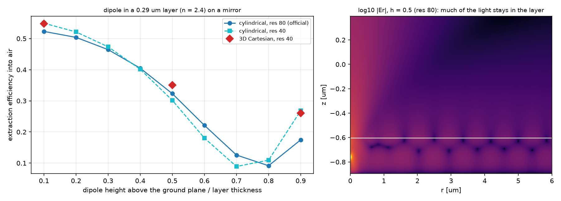 파트 A. 왼쪽: 쌍극자 높이에 따른 추출 효율. cylindrical res 80(파랑), res 40(하늘색), 3D res 40(빨간 마름모). 오른쪽: h = 0.5의 log|Er|. 흰 사각형이 층이고, 층을 따라 멀리까지 가는 빛이 갇힌 몫이다.
| h | CYL res 80 | CYL res 40 | 3D res 40 | 노트: 3D res 80 |
|---|---|---|---|---|
| 0.1 | 0.5230 | 0.5494 | 0.5475 | — |
| 0.2 | 0.5038 | 0.5214 | — | — |
| 0.3 | 0.4645 | 0.4735 | — | — |
| 0.4 | 0.4050 | 0.4014 | — | — |
| 0.5 | 0.3232 | 0.3018 | 0.3505 | 0.3369 |
| 0.6 | 0.2213 | 0.1805 | — | — |
| 0.7 | 0.1259 | 0.0891 | — | — |
| 0.8 | 0.0915 | 0.1095 | — | — |
| 0.9 | 0.1745 | 0.2681 | 0.2607 | — |
파트 B. 왼쪽: r = 3.5 µm 쌍극자의 m 항별 방사 power(그때까지의 최대로 나눔). 빨간 점선이 공식 종료 기준 1%, 회색 점선이 $m=2\pi nr$. 오른쪽: m을 어디서 끊느냐에 따른 효율. 보라 점선은 같은 층에서 축 위 쌍극자의 효율.
| 계산 | m 범위 | 추출 효율 |
|---|---|---|
| 축 위 쌍극자 (r = 0.03 µm, m = 1) | 1 run | 0.3636 |
| r = 3.5 µm, 공식 규칙(첫 1% 미만) | 0…32 | 0.6323 |
| r = 3.5 µm, m = 60까지 | 0…60 | 0.3616 |
| 공식 규칙 뒤의 되튐 | m = 41에서 최대의 0.38 | — |
| 노트(10_sources): 공식 문서 CYL / 3D 기준 | — | 0.320–0.324 / 0.334 |
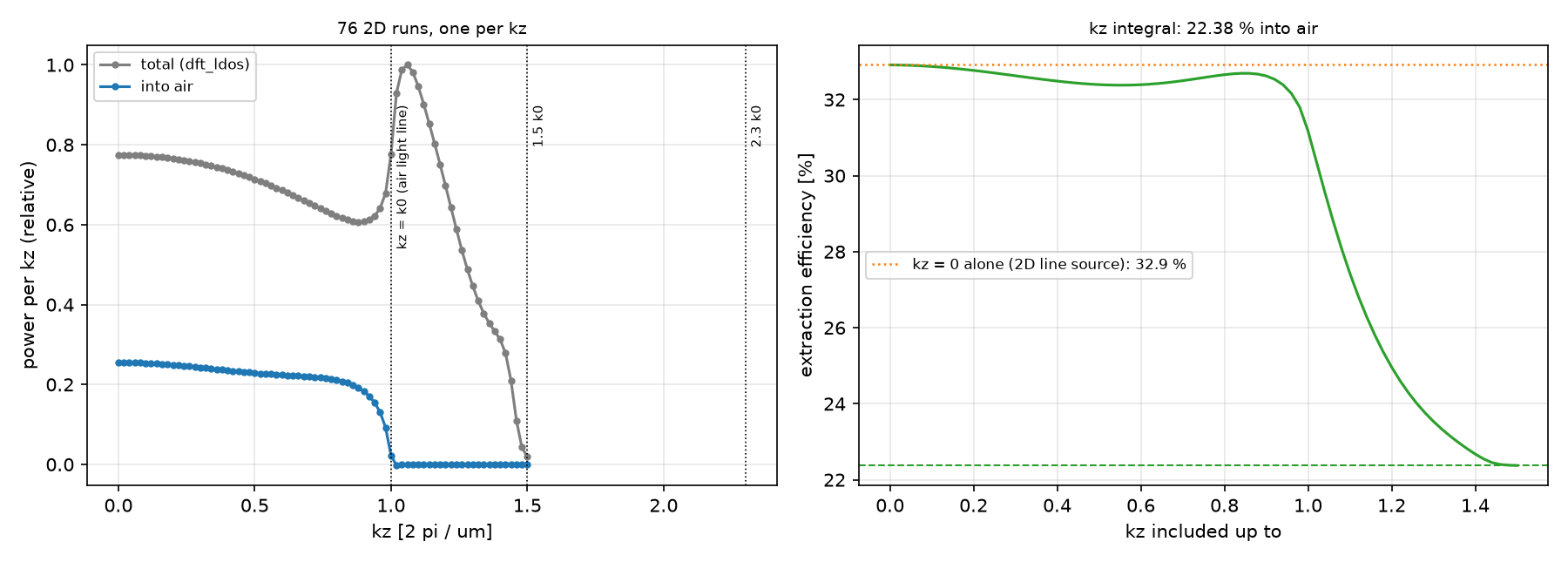 파트 C. 왼쪽: kz마다의 전체 방출(회색)과 공기로 나간 몫(파랑). 점선은 공기, 클래딩, 활성층의 빛선(light line). 오른쪽: kz를 어디까지 더했느냐에 따른 효율.
| 항목 | 값 |
|---|---|
| kz 점 수 | 76 (0~1.50, 간격 0.02) |
| 마지막 kz의 전체 power / 최대 | 0.0189 |
| 추출 효율 (kz 적분) | 22.375% |
| kz = 0 하나만 (2D 선전류) | 32.91% |
| 노트(10_sources) | 22.375%, 76점 |
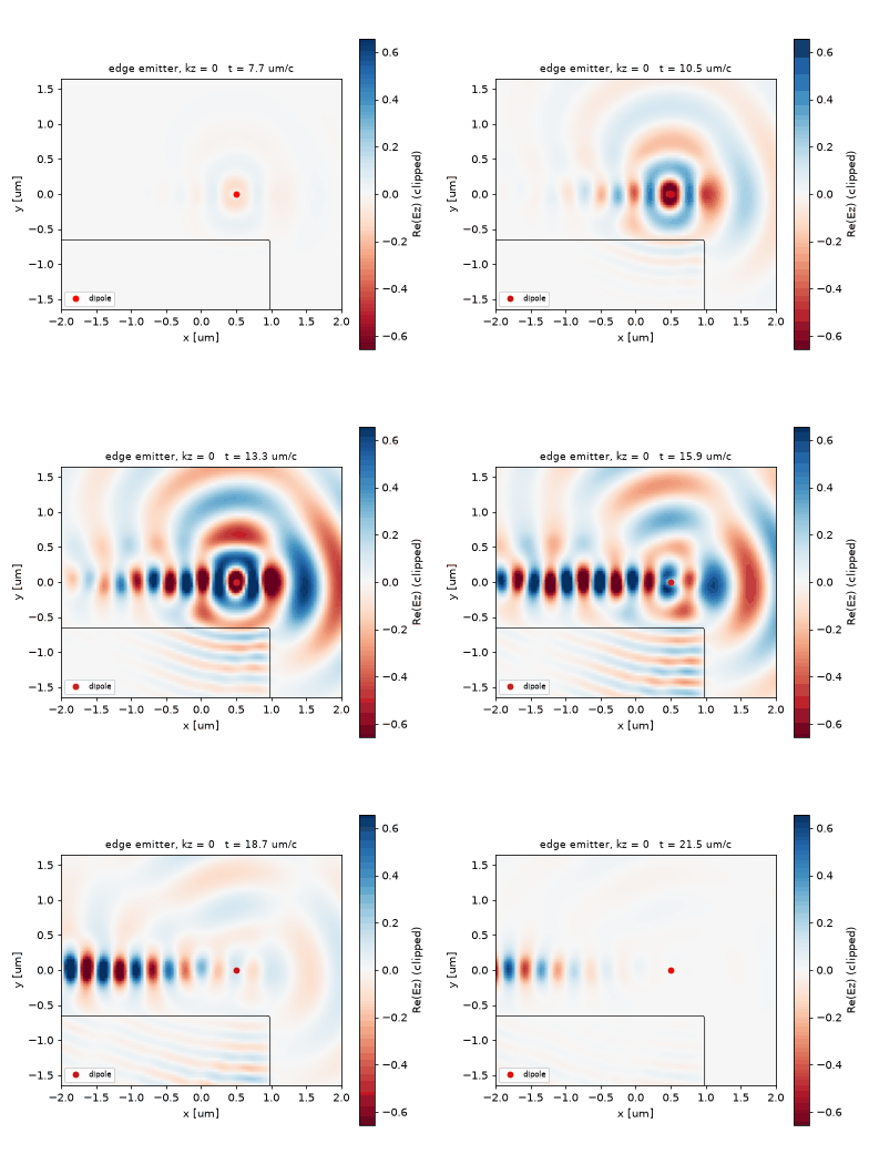 파트 C, kz = 0의 짧은 펄스. 활성층의 쌍극자(빨강)에서 나온 빛 대부분이 다층을 따라 기판 쪽으로 가고, 일부가 절단면을 지나 공기로 나간다.
예측과 비교
| 물리량 | 내 예측 (§2) | 시뮬레이션 | 판정 |
|---|---|---|---|
| 추출 효율(A, h = 0.5) | 0.3 근처 | 0.323 (CYL res 80) | ✅ |
| 높이 의존 | 거울에서 멀수록 변한다 | 0.52 → 0.09(h 0.8) → 0.17 | ✅ |
| CYL res 40 vs 80 | 1% 안 | h ≤ 0.4에서 2~5%, h ≥ 0.6에서 18~54% | ❌ |
| 3D vs CYL | 2% 안 | res 40: h 0.1 0.4%, h 0.5 16%, h 0.9 2.7% | ❌ |
| 축 위 쌍극자(B) | 0.3 근처 | 0.364 | ✅ |
| B: 공식 종료 규칙 | sum-to-60과 다르다 | 0.632 vs 0.362 | ✅ |
| C: 필요한 kz 수 | 70~80 | 76 | ✅ |
| C: 추출 효율 | 22% 근처 | 22.375% | ✅ |
여덟 예측 중 여섯이 맞았고, 틀린 두 개가 모두 해상도 문제였다. 층 두께 0.292 µm는 res 40에서 11.7칸이다. 쌍극자 높이를 층 두께의 비율로 주면 격자에 맞춰 반올림되고, 위쪽 공기 계면 근처(h ≥ 0.6)에서는 field가 급하게 변해 한두 칸의 차이가 효율을 크게 바꾼다. res 40에서 CYL과 3D가 h = 0.5에서 16% 다른 것도 같은 원인으로 본다. 노트의 res 80 값은 CYL 0.323, 3D 0.337로 차이가 1.4%까지 줄었다. 이 층에는 res 80이 필요하다. B는 노트와 소수 넷째 자리까지 같다. 공식 규칙은 m = 32에서 멈춰 0.632를 내지만, 그 뒤 m = 41 근처에서 항이 다시 커진다. 이 항들은 source의 일(분모)이 매우 크고 공기로 나간 몫(분자)은 작다. 층에 갇혀 반지름 방향으로 가는 빛은 쌍극자에서 r만큼 떨어진 곳에서 둘레 $2\pi r$에 $n_{\mathrm{eff}}$배의 파장이 들어가는 m, 즉 $m\approx2\pi n_{\mathrm{eff}}r$ 근처에 실린다. 이 m을 빼면 분모의 대부분이 빠지므로 효율이 두 배로 나온다. m = 60까지 더한 0.362는 축 위 쌍극자의 0.364와 0.5% 안에서 같다. 무한한 층에서는 쌍극자의 가로 위치가 효율을 바꾸지 않아야 하므로 이 일치가 급수를 맞게 끊었다는 검산이다. C에서 kz = 0 하나(2D 선전류)는 32.9%를 주지만 적분하면 22.4%다. kz가 공기의 빛선 k₀를 넘으면 공기로는 빛이 못 나가고(파랑이 0) 다층 안의 guided 방출만 남는다(회색 봉우리). 2D 계산 하나로 3D 소자의 추출 효율을 말하면 이 몫이 빠진다.
수렴성
| 변수 | 값 | 결과 | 비고 |
|---|---|---|---|
| A 해상도 | CYL 40 / 80 (노트 80) | h 0.5: 0.302 / 0.323 | 층이 12칸뿐인 res 40은 부족 |
| A 좌표계 | CYL 40 vs 3D 40; 노트 CYL 80 vs 3D 80 | 16% / 1.4% (h 0.5) | 해상도를 올리면 두 좌표계가 만난다 |
| B m 범위 | 0…32 / 0…60 | 0.632 / 0.362 | 마지막 항 2e-8 |
| C kz 범위 | 0 / 0…1.50 | 32.9% / 22.4% | tail 0.019 |
주장할 수 있는 것 / 없는 것
- 할 수 있는 것: 이 층(n 2.4, 0.7λ/n, 거울 위)에서 수평 쌍극자의 추출 효율은 높이에 따라 0.52에서 0.09까지 변하고, h = 0.5에서 res 80의 cylindrical 값은 0.323이다. 축에서 3.5 µm 떨어진 쌍극자도 m을 guided 빛 너머(60)까지 더하면 축 위와 같은 0.36이 된다. 절단면 레이저(z 쌍극자, 0.5 µm)의 추출 효율은 kz 적분으로 22.4%다.
- 할 수 없는 것: res 40의 높이 곡선(특히 h ≥ 0.6). 3D 값의 수렴(이 글은 res 40만 돌렸다). B의 0.36이 A의 0.32와 다른 이유(셀 크기 20 vs 6 µm, 해상도 50 vs 80, 대역폭이 다르다)를 하나로 정하는 것. 열린 면이라 갇힌 빛이 흡수 없이 어디로 가는지의 에너지 수지.
6. 흔한 실수
| 증상 | 원인 | 고치는 법 |
|---|---|---|
| 효율이 1보다 큼 또는 수백 배 다름 | 분모의 $\Delta V$ 누락, 좌표계에 맞지 않는 $\Delta V$ | cyl $2\pi r/\mathrm{res}^2$, 3D $1/\mathrm{res}^3$, 2D $1/\mathrm{res}^2$ |
| 분모를 진공 source power로 둠 | 거울·층이 방출량을 바꾼다는 것을 잊음 | 같은 run의 dft_ldos로 잰다 |
| 효율이 너무 큼 | 옆면 monitor를 층 높이까지 내림 | 옆면은 공기 높이만 |
| CYL이 축 근처에서 틀림 | Er을 r = 0에 둠 | 1.5 픽셀 offset |
| m 급수 효율이 크게 다름 | 첫 1% 교차에서 멈춤 | guided 빛의 $m\approx2\pi nr$ 너머까지 보고 정한다 |
| kz 적분이 작게 나옴 | kz > 0 항을 두 배로 세지 않음 | ±kz 대칭, $w=2$ |
| 3D가 CYL과 2배 다름 | 3D 대칭 위상 틀림 | Ex는 Mirror(X, −1) |
7. 직접 해보기
| 바꿀 것 | 예상 변화 | 확인할 수치 |
|---|---|---|
| A의 층 두께 0.7λ/n → 0.4λ/n | guided mode가 줄어 효율이 오른다 | η(h = 0.5) |
| A를 수직 쌍극자(Ez, m = 0)로 | 위로 덜 나가 효율이 크게 준다 | η |
| B의 r = 6.7, 9.5 µm | 되튐이 더 큰 m으로 간다 | m_stop, 되튐 위치 |
| C를 x·y 편광으로 | 편광마다 다른 효율 | η |
| 11개 쌍극자 디스크(disc_extraction_efficiency.py) | 노트: 0.932, m 93개 run | η, 마지막 m의 몫 |
8. 전체 코드
code/extraction_efficiency.py 전체 (클릭하여 펼치기)
"""Meep Example 14 - A point source in a thin film: the share that escapes into air (light-extraction efficiency).

Post 11 measured how much a dipole emits (LDOS); post 13 split a body of revolution into m runs. An LED asks
the ratio of the two: of all the power a dipole in the emitting layer puts out, how much reaches the air?
    extraction efficiency = P_air (flux through an open surface in air) / P_total (source work from dft_ldos)
  A. Official extraction_eff_ldos.py: a dipole in a dielectric layer (n = 2.4, t = 0.7 wl / n) on a ground
     plane, efficiency vs dipole height, in cylindrical coordinates (Er, m = -1) at resolution 40 and 80 and in
     3D (Ex) at resolution 40. The denominator needs the voxel volume of each coordinate system.
  B. Official point_dipole_cyl.py: the same slab, a dipole 3.5 um off the axis = an m series. The official stop
     rule (first m whose radiated flux < 1 % of the running max) is compared with summing far beyond it: the
     slab-guided light reaches the side monitor through high m and the series rebounds.
  C. Official edge_emitter_2D.py: a z-dipole 0.5 um inside the cleaved facet of a multilayer laser stack.
     The 3D problem is a 2D cross-section plus an integral over the out-of-plane wavevector kz.
MPI-safe: collective calls on every rank, figures on the master only.

Run:  mpirun -np 4 python extraction_efficiency.py      (~40 min)
Out:  00_source.png, 01_layout.png, 02_layout_edge.png, 03_height.png, 04_m_series.png, 05_kz.png,
      06_field.png, 07_anim_edge.gif, result.json   (-> ../assets/14/)
"""
import json
import math
import os
import sys
import time

import numpy as np
import matplotlib
matplotlib.use("Agg")
import matplotlib.pyplot as plt
import meep as mp

sys.path.insert(0, os.path.dirname(os.path.abspath(__file__)))
from blogfig import Label, animate_fields, annotated_layout, record_frames, source_figure   # noqa: E402

HERE = os.path.dirname(os.path.abspath(__file__))
OUT = os.path.join(HERE, "..", "assets", "14")
os.makedirs(OUT, exist_ok=True)
MASTER = mp.am_master()
t_all = time.time()


def say(*a):
    if MASTER:
        print(*a, flush=True)


def orient_rz(arr, nr):
    arr = np.asarray(arr)
    if arr.ndim == 2 and abs(arr.shape[1] - nr) < abs(arr.shape[0] - nr):
        return arr.T
    return arr


def source_work(sim, dV):
    """Total power emitted by the point source: -Re(F J*) dV from the dft_ldos data."""
    return float(-np.real(sim.ldos_Fdata[0] * np.conj(sim.ldos_Jdata[0])) * dV)


# ================================================================ A. dipole in a layer on a ground plane: CYL vs 3D
WL, FREQ, N_L = 1.0, 1.0, 2.4
T_L = 0.7 * WL / N_L                      # layer thickness
DPML, DAIR, L = 0.5, 1.0, 6.0             # PML, air above the layer, lateral size of the collection surface
TOL = 1e-8
HEIGHTS = np.round(np.linspace(0.1, 0.9, 9), 3)      # dipole height above the ground plane, fraction of T_L
H3D = (0.1, 0.5, 0.9)


def layer(sz):
    return [mp.Block(material=mp.Medium(index=N_L), center=mp.Vector3(0, 0, -0.5 * sz + 0.5 * T_L), size=mp.Vector3(mp.inf, mp.inf, T_L))]


def eff_cyl(h, res, want=False):
    sr, sz = L + DPML, T_L + DAIR + DPML
    src_pt = mp.Vector3(1.5 / res, 0, -0.5 * sz + h * T_L)          # Er at r = 0 is undefined on the Yee grid (meep #2704)
    sim = mp.Simulation(resolution=res, cell_size=mp.Vector3(sr, 0, sz), dimensions=mp.CYLINDRICAL, m=-1,
                        boundary_layers=[mp.PML(DPML, direction=mp.R), mp.PML(DPML, direction=mp.Z, side=mp.High)],   # bottom: no PML = ground plane
                        sources=[mp.Source(mp.GaussianSource(FREQ, fwidth=0.1 * FREQ), component=mp.Er, center=src_pt)], geometry=layer(sz))
    flux = sim.add_flux(FREQ, 0, 1, mp.FluxRegion(center=mp.Vector3(0.5 * L, 0, 0.5 * sz - DPML), size=mp.Vector3(L, 0, 0)),
                        mp.FluxRegion(center=mp.Vector3(L, 0, 0.5 * sz - DPML - 0.5 * DAIR), size=mp.Vector3(0, 0, DAIR)))
    dft = sim.add_dft_fields([mp.Er], FREQ, 0, 1, center=mp.Vector3(0.5 * L, 0, -0.5 * DPML), size=mp.Vector3(L, 0, sz - DPML)) if want else None
    if want:
        annotated_layout(sim, os.path.join(OUT, "01_layout.png"), dpml=DPML, figsize=(11, 3.6), axis_step=1.0, unit="um",
                         title="part A, cylindrical (r, z) cell: dipole in a layer (n = 2.4) on a ground plane; x = r, y = z",
                         params_text=f"wl={WL} um, res={res}\nt = 0.7 wl/n = {T_L:.3f} um", params_xy=(3.6, 0.33), pml_xy=(6.05, -0.6),
                         decay_point=(src_pt.x, src_pt.z), decay_text_xy=(1.8, -0.45),
                         labels=[Label("layer n = 2.4 (bottom edge: PEC ground plane, no PML)", (2.5, -0.75), (1.8, -0.2), step=2, color="black"),
                                 Label("Er dipole at r = 1.5 px, height h", (src_pt.x, src_pt.z), (1.8, 0.05), step=3, color="red"),
                                 Label("numerator: flux through top + outer r (air only)", (4.0, 0.5 * sz - DPML), (3.6, -0.2), step=5, color="blue")])
    sim.run(mp.dft_ldos(FREQ, 0, 1), until_after_sources=mp.stop_when_fields_decayed(20, mp.Er, src_pt, TOL))
    p_air = float(mp.get_fluxes(flux)[0])
    p_tot = source_work(sim, 2 * np.pi * src_pt.x / res ** 2)         # CYL voxel: 2 pi r dr dz
    er = orient_rz(sim.get_dft_array(dft, mp.Er, 0), int(round(L * res))) if want else None
    sim.reset_meep()
    return p_air / p_tot, er, sz


def eff_3d(h, res):
    sxy, sz = L + 2 * DPML, T_L + DAIR + DPML
    src_pt = mp.Vector3(0, 0, -0.5 * sz + h * T_L)
    sim = mp.Simulation(resolution=res, cell_size=mp.Vector3(sxy, sxy, sz), symmetries=[mp.Mirror(mp.X, phase=-1), mp.Mirror(mp.Y)],
                        boundary_layers=[mp.PML(DPML, direction=mp.X), mp.PML(DPML, direction=mp.Y), mp.PML(DPML, direction=mp.Z, side=mp.High)],
                        sources=[mp.Source(mp.GaussianSource(FREQ, fwidth=0.1 * FREQ), component=mp.Ex, center=src_pt)], geometry=layer(sz))
    zc = 0.5 * sz - DPML - 0.5 * DAIR
    flux = sim.add_flux(FREQ, 0, 1, mp.FluxRegion(center=mp.Vector3(0, 0, 0.5 * sz - DPML), size=mp.Vector3(L, L, 0)),
                        mp.FluxRegion(center=mp.Vector3(0.5 * L, 0, zc), size=mp.Vector3(0, L, DAIR)),
                        mp.FluxRegion(center=mp.Vector3(-0.5 * L, 0, zc), size=mp.Vector3(0, L, DAIR), weight=-1.0),
                        mp.FluxRegion(center=mp.Vector3(0, 0.5 * L, zc), size=mp.Vector3(L, 0, DAIR)),
                        mp.FluxRegion(center=mp.Vector3(0, -0.5 * L, zc), size=mp.Vector3(L, 0, DAIR), weight=-1.0))
    sim.run(mp.dft_ldos(FREQ, 0, 1), until_after_sources=mp.stop_when_fields_decayed(20, mp.Ex, src_pt, TOL))
    p_air = float(mp.get_fluxes(flux)[0])
    p_tot = source_work(sim, 1 / res ** 3)                                # 3D voxel
    sim.reset_meep()
    return p_air / p_tot


t_a = time.time()
effA = {"cyl40": [], "cyl80": []}
er_map, sz_A = None, None
for h in HEIGHTS:
    effA["cyl40"].append(eff_cyl(h, 40)[0])
    e80, er, sz = eff_cyl(h, 80, want=(h == 0.5))
    effA["cyl80"].append(e80)
    if er is not None:
        er_map, sz_A = er, sz
say("A (cyl): " + "; ".join(f"h {h:.1f}: res40 {a:.4f}, res80 {b:.4f}" for h, a, b in zip(HEIGHTS, effA["cyl40"], effA["cyl80"])) + f"; {time.time() - t_a:.0f} s")
t_a3 = time.time()
eff3 = {h: eff_3d(h, 40) for h in H3D}
say("A (3D, res 40): " + "; ".join(f"h {h}: {v:.4f} (cyl40 {effA['cyl40'][list(HEIGHTS).index(h)]:.4f}, cyl80 {effA['cyl80'][list(HEIGHTS).index(h)]:.4f})" for h, v in eff3.items()) + f"; {time.time() - t_a3:.0f} s")
if MASTER:
    source_figure(FREQ, 0.1 * FREQ, os.path.join(OUT, "00_source.png"), wl_scale=1000.0, wl_unit="nm", time_unit="um/c")

# ================================================================ B. off-axis dipole in the slab: the m series and when to stop
t_b = time.time()
RES_B, R_CELL, PML_B, PAD_B = 50, 20.0, 1.0, 1.0
M_MAX = 60
R_SRC = 3.5


def dipole_in_slab(rpos, m):
    sr, sz = R_CELL + PML_B, T_L + PAD_B + PML_B
    src_pt = mp.Vector3(rpos, 0, -0.5 * sz + 0.5 * T_L)
    sim = mp.Simulation(resolution=RES_B, cell_size=mp.Vector3(sr, 0, sz), dimensions=mp.CYLINDRICAL, m=m, force_complex_fields=True,
                        boundary_layers=[mp.PML(PML_B, direction=mp.R), mp.PML(PML_B, direction=mp.Z, side=mp.High)],
                        sources=[mp.Source(mp.GaussianSource(FREQ, fwidth=0.05 * FREQ), component=mp.Er, center=src_pt)], geometry=layer(sz))
    flux = sim.add_flux(FREQ, 0, 1, mp.FluxRegion(center=mp.Vector3(0.5 * R_CELL, 0, 0.5 * sz - PML_B), size=mp.Vector3(R_CELL, 0, 0)),
                        mp.FluxRegion(center=mp.Vector3(R_CELL, 0, 0.5 * sz - PML_B - 0.5 * PAD_B), size=mp.Vector3(0, 0, PAD_B)))
    sim.run(mp.dft_ldos(FREQ, 0, 1), until_after_sources=mp.stop_when_dft_decayed(tol=1e-4))
    rad = float(mp.get_fluxes(flux)[0])
    src = source_work(sim, 2 * np.pi * rpos / RES_B ** 2)
    sim.reset_meep()
    return rad, src


r_ax = 1.5 / RES_B
rad_ax, src_ax = dipole_in_slab(r_ax, 1)
eff_axis = rad_ax / src_ax
say(f"B: dipole on the axis (m = 1, r = {r_ax:.2f}): extraction {eff_axis:.4f}")
rads, srcs = [], []
for m in range(M_MAX + 1):
    rad, src = dipole_in_slab(R_SRC, m)
    rads.append(rad); srcs.append(src)
    if m % 5 == 0:
        say(f"B: r {R_SRC}, m = {m}: radiated {rad:.4e}, source {src:.4e}; {time.time() - t_b:.0f} s")
rads, srcs = np.array(rads), np.array(srcs)
w = np.where(np.arange(M_MAX + 1) == 0, 1, 2)                                  # +-m give the same power: count m > 0 twice
running_max = np.maximum.accumulate(rads)
rel = rads / running_max
m_stop = int(next(m for m in range(1, M_MAX + 1) if rel[m] < 1e-2))             # official rule: first m > 0 below 1 % of the running max
eff_series = np.cumsum(w * rads) / np.cumsum(w * srcs)
eff_official = float(eff_series[m_stop]); eff_full = float(eff_series[-1])
rebound = float(rel[m_stop:].max())
m_rebound = int(m_stop + np.argmax(rel[m_stop:]))
say(f"B: official stop at m = {m_stop} (radiated/max {rel[m_stop]:.2e}) -> efficiency {eff_official:.4f}; after the stop the series rebounds to "
    f"{rebound:.3f} of the max at m = {m_rebound}; summed to m = {M_MAX}: efficiency {eff_full:.4f} (last term {rel[-1]:.1e}); {time.time() - t_b:.0f} s")

# ================================================================ C. cleaved-facet edge emitter: 2D cross-section + kz integral
t_c = time.time()
RES_C, CLAD, ACT, SUB, PML_C, AIR_C, SIDE = 25, 0.5, 0.3, 1.0, 0.5, 1.0, 3.0
N_SUB, N_CLAD, N_ACT = 3.2, 1.5, 2.3
DKZ, KZ_TOL, POS_C = 0.02, 0.02, 0.5
CX = PML_C + SIDE + AIR_C + PML_C
CY = PML_C + SUB + CLAD + ACT + CLAD + AIR_C + PML_C
SRC_C = mp.Vector3(-0.5 * CX + PML_C + SIDE - POS_C, -0.5 * CY + PML_C + SUB + CLAD + 0.5 * ACT)


def stack():
    x0 = -0.5 * CX + 0.5 * (PML_C + SIDE); wx = PML_C + SIDE; y = -0.5 * CY
    out = []
    for th, n in ((PML_C + SUB, N_SUB), (CLAD, N_CLAD), (ACT, N_ACT), (CLAD, N_CLAD)):
        out.append(mp.Block(material=mp.Medium(index=n), center=mp.Vector3(x0, y + 0.5 * th), size=mp.Vector3(wx, th, mp.inf))); y += th
    return out


def edge_sim(kz, fwidth=0.1 * FREQ, monitors=True):
    sim = mp.Simulation(resolution=RES_C, cell_size=mp.Vector3(CX, CY), k_point=mp.Vector3(0, 0, kz), kz_2d="real/imag",
                        sources=[mp.Source(mp.GaussianSource(FREQ, fwidth=fwidth), component=mp.Ez, center=SRC_C)], geometry=stack(),
                        boundary_layers=[mp.PML(PML_C)])
    flux = None
    if monitors:
        flux = sim.add_flux(FREQ, 0, 1,
                            mp.FluxRegion(center=mp.Vector3(0, 0.5 * CY - PML_C), size=mp.Vector3(CX - 2 * PML_C, 0)),                 # top
                            mp.FluxRegion(center=mp.Vector3(0.5 * CX - PML_C, 0), size=mp.Vector3(0, CY - 2 * PML_C)),                 # right (in front of the facet)
                            mp.FluxRegion(center=mp.Vector3(0.5 * CX - PML_C - 0.5 * AIR_C, -0.5 * CY + PML_C), size=mp.Vector3(AIR_C, 0), weight=-1.0))   # bottom of the air gap
    return sim, flux


kzs, d_kz, a_kz = [], [], []
nkz, dmax = 0, 0.0
while True:
    kz = nkz * DKZ
    sim, flux = edge_sim(kz)
    if nkz == 0:
        annotated_layout(sim, os.path.join(OUT, "02_layout_edge.png"), dpml=PML_C, figsize=(6.4, 6.0), axis_step=1.0, unit="um",
                         title="part C: cleaved facet of a laser stack (2D x-y); the stack is uniform along z",
                         params_text=f"res={RES_C}, kz step {DKZ}\nsub 3.2 / clad 1.5 / act 2.3", params_xy=(-2.4, 2.25), pml_xy=(-2.4, -2.2), decay_point=None,
                         labels=[Label("Ez dipole 0.5 um inside the facet", (SRC_C.x, SRC_C.y), (-2.4, 1.5), step=3, color="red"),
                                 Label("active layer n = 2.3 between claddings", (-1.5, SRC_C.y), (-2.4, 0.8), step=2, color="black"),
                                 Label("air flux: top + front + under the gap", (1.9, 0.6), (-0.3, 1.9), step=5, color="blue")])
    sim.run(mp.dft_ldos(FREQ, 0, 1), until_after_sources=mp.stop_when_fields_decayed(25, mp.Ez, SRC_C, 1e-6))
    dflux = source_work(sim, 1 / RES_C ** 2)            # 2D: a line current, pixel area
    aflux = float(mp.get_fluxes(flux)[0])
    sim.reset_meep()
    kzs.append(kz); d_kz.append(dflux); a_kz.append(aflux)
    nkz += 1
    if dflux > dmax:
        dmax = dflux
    elif dflux / dmax < KZ_TOL:
        break
kzs, d_kz, a_kz = map(np.array, (kzs, d_kz, a_kz))
eff_edge = float((a_kz[0] + 2 * a_kz[1:].sum()) / (d_kz[0] + 2 * d_kz[1:].sum()))
eff_kz0 = float(a_kz[0] / d_kz[0])
kz_cut = N_ACT * FREQ
say(f"C: {len(kzs)} kz points up to {kzs[-1]:.2f} (tail {d_kz[-1] / dmax:.4f}); extraction {100 * eff_edge:.3f} % (kz = 0 alone: {100 * eff_kz0:.2f} %); {time.time() - t_c:.0f} s")

# GIF: kz = 0, short pulse, monitor-free
sim_g, _ = edge_sim(0.0, fwidth=0.4 * FREQ, monitors=False)
sim_g.init_sim()
vol = mp.Volume(center=mp.Vector3(), size=mp.Vector3(CX - 2 * PML_C, CY - 2 * PML_C))
eps_g = sim_g.get_array(vol=vol, component=mp.Dielectric)
t0 = 5 / (0.4 * FREQ)
frames, times = record_frames(sim_g, vol, mp.Ez, t_start=t0 - 2 / (0.4 * FREQ), t_end=t0 + 9.0, n_frames=60)
sim_g.reset_meep()

# ================================================================ figures
if MASTER:
    fig, ax = plt.subplots(1, 2, figsize=(12, 4.3), gridspec_kw={"width_ratios": [1.4, 1]})
    ax[0].plot(HEIGHTS, effA["cyl80"], "o-", color="tab:blue", label="cylindrical, res 80 (official)")
    ax[0].plot(HEIGHTS, effA["cyl40"], "s--", color="tab:cyan", label="cylindrical, res 40")
    ax[0].plot(list(H3D), [eff3[h] for h in H3D], "D", color="tab:red", ms=8, label="3D Cartesian, res 40")
    ax[0].set_xlabel("dipole height above the ground plane / layer thickness"); ax[0].set_ylabel("extraction efficiency into air")
    ax[0].set_title("dipole in a 0.29 um layer (n = 2.4) on a mirror", fontsize=9); ax[0].grid(alpha=0.3); ax[0].legend(fontsize=8)
    ext = [0, L, -0.5 * sz_A, 0.5 * sz_A - DPML]
    ax[1].imshow(np.log10(np.abs(er_map) + 1e-12).T, extent=ext, origin="lower", cmap="inferno", aspect="auto")
    ax[1].add_patch(plt.Rectangle((0, -0.5 * sz_A), L, T_L, fill=False, color="w", lw=1))
    ax[1].set_xlabel("r [um]"); ax[1].set_ylabel("z [um]"); ax[1].set_title("log10 |Er|, h = 0.5 (res 80): much of the light stays in the layer", fontsize=9)
    fig.tight_layout(); fig.savefig(os.path.join(OUT, "03_height.png"), dpi=150); plt.close(fig)

    ms = np.arange(M_MAX + 1)
    fig, ax = plt.subplots(1, 2, figsize=(12, 4.3))
    ax[0].semilogy(ms, rel, "o-", ms=3, color="tab:blue", label="radiated(m) / running max")
    ax[0].axhline(1e-2, color="crimson", ls="--", lw=1, label="official stop: 1 %")
    ax[0].axvline(m_stop, color="crimson", ls=":", lw=1); ax[0].text(m_stop + 0.5, 2e-1, f"stop at m = {m_stop}", color="crimson", fontsize=8)
    ax[0].plot(m_rebound, rebound, "*", color="tab:orange", ms=12, label=f"rebound {rebound:.2f} at m = {m_rebound}")
    ax[0].axvline(2 * np.pi * N_L * R_SRC, color="gray", ls="-.", lw=1); ax[0].text(2 * np.pi * N_L * R_SRC - 14, 2e-4, "m = 2 pi n r (guided in the slab)", fontsize=8, color="gray")
    ax[0].set_xlabel("azimuthal order m"); ax[0].set_ylabel("radiated power of the m term (relative)"); ax[0].set_title(f"dipole at r = {R_SRC} um in the slab", fontsize=9); ax[0].grid(alpha=0.3, which="both"); ax[0].legend(fontsize=7)
    ax[1].plot(ms, eff_series, "-", color="tab:green"); ax[1].axvline(m_stop, color="crimson", ls=":", lw=1)
    ax[1].axhline(eff_axis, color="tab:purple", ls="--", lw=1, label=f"dipole on the axis: {eff_axis:.3f}")
    ax[1].plot(m_stop, eff_official, "o", color="crimson", label=f"official stop: {eff_official:.3f}")
    ax[1].plot(M_MAX, eff_full, "o", color="tab:green", label=f"summed to m = {M_MAX}: {eff_full:.3f}")
    ax[1].set_xlabel("m included up to"); ax[1].set_ylabel("extraction efficiency"); ax[1].set_title("the efficiency depends on where the series is cut", fontsize=9); ax[1].grid(alpha=0.3); ax[1].legend(fontsize=7)
    fig.tight_layout(); fig.savefig(os.path.join(OUT, "04_m_series.png"), dpi=150); plt.close(fig)

    fig, ax = plt.subplots(1, 2, figsize=(12, 4.3))
    ax[0].plot(kzs, d_kz / d_kz.max(), "o-", ms=3, color="tab:gray", label="total (dft_ldos)")
    ax[0].plot(kzs, a_kz / d_kz.max(), "o-", ms=3, color="tab:blue", label="into air")
    for kc, lab in ((FREQ, "kz = k0 (air light line)"), (N_CLAD * FREQ, "1.5 k0"), (N_ACT * FREQ, "2.3 k0")):
        ax[0].axvline(kc, color="k", ls=":", lw=0.8); ax[0].text(kc + 0.02, 0.9, lab, fontsize=7, rotation=90, va="top")
    ax[0].set_xlabel("kz [2 pi / um]"); ax[0].set_ylabel("power per kz (relative)"); ax[0].set_title(f"{len(kzs)} 2D runs, one per kz", fontsize=9); ax[0].grid(alpha=0.3); ax[0].legend(fontsize=8)
    cum = (np.cumsum(np.where(np.arange(len(kzs)) == 0, 1, 2) * a_kz)) / (np.cumsum(np.where(np.arange(len(kzs)) == 0, 1, 2) * d_kz))
    ax[1].plot(kzs, 100 * cum, "-", color="tab:green"); ax[1].axhline(100 * eff_edge, color="tab:green", ls="--", lw=1)
    ax[1].axhline(100 * eff_kz0, color="tab:orange", ls=":", lw=1.2, label=f"kz = 0 alone (2D line source): {100 * eff_kz0:.1f} %")
    ax[1].set_xlabel("kz included up to"); ax[1].set_ylabel("extraction efficiency [%]"); ax[1].set_title(f"kz integral: {100 * eff_edge:.2f} % into air", fontsize=9); ax[1].grid(alpha=0.3); ax[1].legend(fontsize=8)
    fig.tight_layout(); fig.savefig(os.path.join(OUT, "05_kz.png"), dpi=150); plt.close(fig)

    animate_fields(frames, times, [-(0.5 * CX - PML_C), 0.5 * CX - PML_C, -(0.5 * CY - PML_C), 0.5 * CY - PML_C], os.path.join(OUT, "07_anim_edge.gif"),
                   eps=eps_g, figsize=(5.6, 5.0), dpi=70, clip_percentile=99.0, points=[(SRC_C.x, SRC_C.y, "red", "dipole")],
                   title="edge emitter, kz = 0", legend_loc="lower left")
    with open(os.path.join(OUT, "result.json"), "w") as f_:
        json.dump({"A": {"heights": HEIGHTS.tolist(), "cyl40": effA["cyl40"], "cyl80": effA["cyl80"], "3d40": {str(k): v for k, v in eff3.items()}},
                   "B": {"r": R_SRC, "eff_axis": eff_axis, "m_stop": m_stop, "eff_official": eff_official, "eff_full": eff_full, "rebound": rebound,
                         "m_rebound": m_rebound, "rel": rel.tolist(), "eff_series": eff_series.tolist()},
                   "C": {"n_kz": len(kzs), "kz_max": float(kzs[-1]), "tail": float(d_kz[-1] / dmax), "eff": eff_edge, "eff_kz0": eff_kz0},
                   "wall_s_total": time.time() - t_all, "np": mp.count_processors(), "meep": mp.__version__}, f_, indent=2)
say(f"total {time.time() - t_all:.0f} s on {mp.count_processors()} process(es)")
§4의 발췌 코드와 달리 전체 코드에는 높이 sweep, m 급수와 종료 규칙 비교, kz 적분, GIF, result.json 기록이 들어 있다. MPI로 돌릴 수 있게 collective 호출은 모든 rank에서, 그림 저장은 master에서만 한다. 설계도 두 장은 시간 진행 없이 같은 셀을 만드는 code/extraction_layouts.py로 그렸다. 전체 코드와 helper: https://github.com/jin-castle/meep-examples/blob/main/code.
실행 결과 (2026-10-23 실행, mpirun -np 4):
A (cyl): h 0.1: res40 0.5494, res80 0.5230; h 0.2: res40 0.5214, res80 0.5038; h 0.3: res40 0.4735, res80 0.4645; h 0.4: res40 0.4014, res80 0.4050; h 0.5: res40 0.3018, res80 0.3232; h 0.6: res40 0.1805, res80 0.2213; h 0.7: res40 0.0891, res80 0.1259; h 0.8: res40 0.1095, res80 0.0915; h 0.9: res40 0.2681, res80 0.1745; 253 s
A (3D, res 40): h 0.1: 0.5475 (cyl40 0.5494, cyl80 0.5230); h 0.5: 0.3505 (cyl40 0.3018, cyl80 0.3232); h 0.9: 0.2607 (cyl40 0.2681, cyl80 0.1745); 476 s
B: dipole on the axis (m = 1, r = 0.03): extraction 0.3636
B: r 3.5, m = 0: radiated 8.3457e+03, source 9.8732e+03
B: r 3.5, m = 20: radiated 1.8285e+03, source 5.9457e+03
B: r 3.5, m = 40: radiated 4.1701e+03, source 3.9968e+04
B: r 3.5, m = 60: radiated 2.4012e-04, source 3.0755e-02
B: official stop at m = 32 (radiated/max 5.48e-03) -> efficiency 0.6323; after the stop the series rebounds to 0.382 of the max at m = 41; summed to m = 60: efficiency 0.3616 (last term 2.0e-08); 3502 s
C: 76 kz points up to 1.50 (tail 0.0189); extraction 22.375 % (kz = 0 alone: 32.91 %); 359 s
total 4604 s on 4 process(es)
재현 환경: meep 1.33.0 (MPI) · Python 3.11 · conda install -c conda-forge pymeep=*=mpi_mpich_* · 실행 mpirun -np 4 python extraction_efficiency.py (약 77 min (mpirun -np 4; B alone 58 min))
확인 질문
- 11편의 Purcell 인자에서는 $\Delta V$가 필요 없었는데 추출 효율에서는 왜 필요한가.
- 축에서 3.5 µm 떨어진 쌍극자의 m 급수가 m 30 근처에서 작아졌다가 다시 커지는 이유를 층에 갇힌 빛과 $m\approx2\pi n r$로 설명해 보라.
- 실제 OLED의 발광층에는 위치와 방향이 제각각인 분자가 수천 개 있고, 서로 위상이 맞지 않는다. 이 글처럼 쌍극자 하나씩 돌려 power를 더하면 run이 몇 개 필요한가. 그것을 몇 번의 run으로 줄이는 방법이 있는가. (15편)
9. 더 읽기
- LDOS 튜토리얼: LED 추출 효율 · nonaxisymmetric dipole sources ·
dft_ldos· kz_2d - 스크립트: extraction_eff_ldos.py · point_dipole_cyl.py · edge_emitter_2D.py · disc_extraction_efficiency.py
- 이전 글: 13 · 회전 대칭으로 3D를 계산하기 · LDOS: 11 · 두 거울 사이의 점광원 · 다음 글: 15 · 점광원이 수천 개일 때