MEEP EXAMPLES 13
회전 대칭으로 3D 빛을 어떻게 계산할까?
방위 차수 m으로 계산을 나누고 쌍극자 field를 합칩니다. 고리의 좌표계 비교와 열린 near2far 면의 한계를 함께 확인합니다.
이 글을 읽고 나면
- source 방향과 위치에 맞는 방위 차수 m을 선택한다.
- field 합산과 m별 power 기준의 역할을 구별한다.
- 고리의 차원과 디스크 near–far 차이의 한계를 해석한다.
먼저 알면 좋은 것 10편 near2far와 방사 패턴 · 12편 고리의 방위 차수 m
1. 먼저 보기: 축에서 벗어난 점광원은 몇 번 계산해야 할까?
회전 대칭인 구조를 계산할 때도 source까지 항상 축 대칭인 것은 아닙니다. 축에서 0.5 µm 떨어진 점광원 하나를 표현하려면, 방위 차수 m을 바꾸어 여러 번 계산한 field를 합쳐야 합니다.
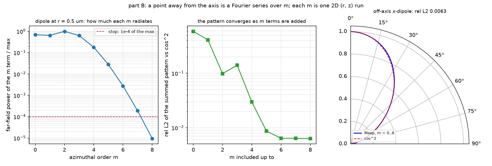
부분합이 매번 좋아지는 것은 아닙니다. m = 0…2의 패턴 오차는 0.099였지만 m = 3을 더하면 0.141로 잠시 증가했습니다. 모양이 좋아 보이는 중간 결과에서 멈추지 말고, m별 power와 패턴을 함께 확인합니다. 다른 구조나 더 먼 source에서는 power가 한 번 작아진 뒤 다시 커질 수도 있습니다.
2. 먼저 예측하기: 회전 대칭 구조면 m = 0만 있으면 될까?
예측과 source 표현 비교하기
두 번째입니다. 구조가 회전 대칭이어도 x 방향은 방위각 φ에 따라 원통좌표의 r·φ 성분이 달라집니다. 이 예제는 m = +1과 −1에서 Er와 ±i Ep를 사용하고 두 field를 반씩 더합니다. 축 위의 z 방향 쌍극자는 m = 0 한 번으로 표현합니다.
3. 원리 이해하기: 방위각을 m으로 나누어 계산하기
구조가 φ에 무관하면 field를 E(r, φ, z) = Σ E_m(r, z) exp(imφ)로 쓸 수 있습니다. m 하나를 고르면 φ 미분은 im을 곱하는 것으로 바뀌고, Meep은 남은 r–z 단면을 계산합니다. 3D 공간의 효과를 버리는 것이 아니라 방위각 의존성을 별도로 표현하는 방법입니다.
| source 또는 문제 | 필요한 표현 |
|---|---|
| 축 위 z 쌍극자 | m = 0, Ez |
| 축 위 x 쌍극자 | m = +1과 −1, Er와 ±i Ep |
| 축 밖 점광원 | 여러 m의 Fourier 급수 |
| 정해진 방위 차수의 고리 모드 | 해당 m 하나로 계산 |
패턴은 field를 더한 뒤 power를 구합니다. φ = 0 단면에서 m별 power만 더하면 항 사이의 간섭이 사라집니다. 반면 전체 방위각에 걸쳐 적분한 총 power는 서로 다른 m의 직교성 때문에 항별 power를 더할 수 있습니다. 이 예제는 m 항의 power가 최대값의 10⁻⁴ 아래인지로 급수 중단을 판단합니다.
이 중단 규칙은 여기의 진공 r₀ = 0.5 µm 예제에 대한 기준입니다. 더 먼 source나 구조가 있는 문제에서 처음으로 작은 항 하나를 발견했다고 이후의 모든 항이 작다고 보장할 수는 없습니다.
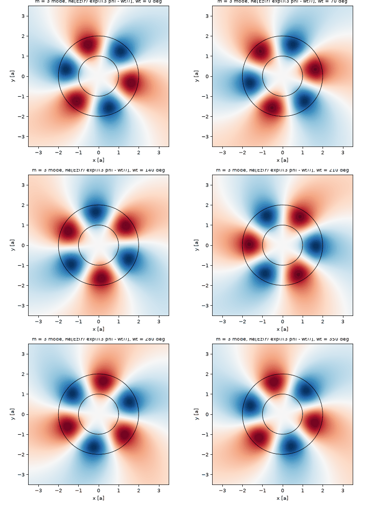
고리 예제의 차원. 파트 C의 ring-cyl은 셀의 z 크기가 0입니다. 12편의 z로 무한한 2D 고리 문제를 다른 좌표로 푼 것으로, 유한 높이의 실제 3D ring을 검증한 것은 아닙니다. 반면 일반적인 cylindrical r–z 셀은 회전 대칭 3D 구조를 m별로 표현할 수 있습니다.
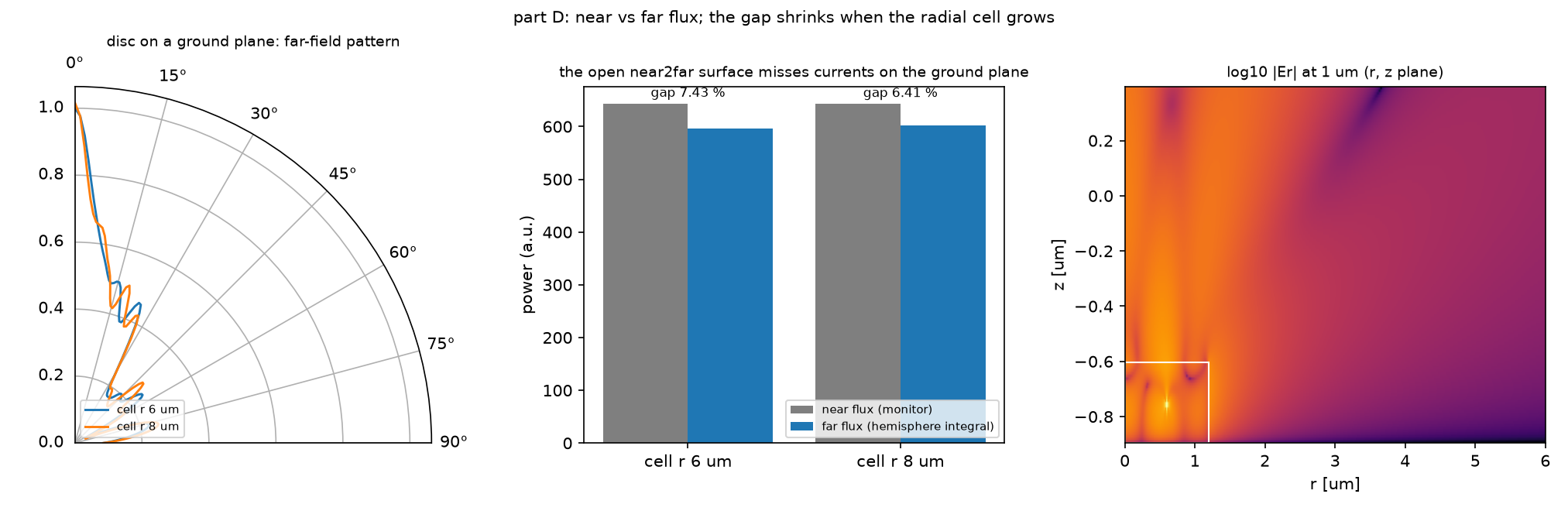
파트 D의 디스크는 굴절률 2.4, 반지름 1.2 µm이고 아래에 손실 없는 PEC ground plane이 있습니다. m = −1 하나의 ring source를 계산하며, 임의의 off-axis 점광원 전체를 계산한 결과는 아닙니다. ground plane 때문에 near2far 면은 위와 바깥 r만 포함하고 아래는 열려 있습니다.
4. 직접 실행하기: m 급수의 중단 기준만 엄격하게 하기
저장소를 내려받아 code/ 폴더에서 실행합니다. cylindrical_dipole.py와 같은 폴더의 blogfig.py가 모두 필요합니다. Meep 1.33.0 MPI 환경과 Python·NumPy·Matplotlib을 사용한 원본 기록은 MPI 4개 프로세스에서 약 7.6분입니다.
OMP_NUM_THREADS=1 mpirun -np 4 python cylindrical_dipole.py
먼저 원본 결과를 별도 폴더에 보관하세요. POWER_DECAY = 1e-4를 1e-5로만 바꾸고 같은 명령으로 다시 실행합니다. source 거리, 해상도, 나머지 파트의 설정은 그대로 둡니다.
파트 B 로그의 마지막 m, 마지막 항의 power 비율, 최종 패턴 오차를 비교합니다. 원본 m = 8의 비율은 이미 9.49e-6이므로 이 한 단계의 기준 변경만으로 마지막 m이 늘지 않을 수도 있습니다. 이를 미리 실패로 판단하지 말고 실제 종료 기록을 확인하세요. 새 측정값은 원본 0.63%와 구별해 기록합니다.
5. 결과 해석하기: 무엇이 일치했고 무엇이 남았을까?
| 원본 비교 | 실제 결과 | 해석 범위 |
|---|---|---|
| 축 위 z 쌍극자 vs sin²θ | 상대 L2 0.43% | φ = 0의 정규화 패턴 |
| 축 위 x 쌍극자 vs cos²θ | 상대 L2 0.46% | m = ±1 field 합산 |
| 축 밖 r₀ = 0.5 µm | m = 0…8, 상대 L2 0.63% | 이 진공 예제의 급수 |
| 고리 m = 3, 4, 5 주파수 | 12편과 약 0.02%, 0.07%, 0.10% 차이 | 같은 2D 문제의 좌표계 비교 |
고리 m = 5의 Q는 cylindrical에서 1627, 12편 Cartesian 해상도 20에서 2132였습니다. 주파수가 가깝다고 Q도 수렴했다고 볼 수 없습니다. 다른 해상도의 Cartesian 값 1675·1610이 cylindrical 쪽에 가깝지만, 이것만으로 차이의 원인을 계단 경계 하나로 확정하지는 않습니다.
| 셀 반지름 | near flux | far flux | 상대 차이 |
|---|---|---|---|
| 6 µm | 643.65 | 595.80 | 7.43% |
| 8 µm | 643.28 | 602.05 | 6.41% |
near flux는 거의 유지되고 far flux가 증가했습니다. 이는 열린 면 바깥의 등가 전류가 잘리는 truncation 해석과 맞지만, 두 셀 크기만으로 참된 far-field 총 power를 확정하지는 못합니다. 7.43%는 광추출 효율이 아니라 두 power 측정의 불일치입니다.
6. 이해 확인하기
- 축 위 x 쌍극자에서 m = 0 한 번으로 충분하지 않은 이유와, 방향별 패턴을 합산하는 순서를 설명해 보세요.
- 디스크의 near–far 차이가 7.43%에서 6.41%로 줄었다면, far-field 총 power가 수렴했다고 말할 수 있나요?
두 질문의 답 확인하기
- x 방향의 원통좌표 성분은 φ에 의존하므로 m = +1과 −1이 필요합니다. 필요한 m들의 복소 field를 먼저 더하고 Poynting으로 패턴을 구해야 간섭을 보존합니다.
- 아닙니다. 열린 near2far 면의 절단 효과가 줄어드는 해석과 일치할 뿐, 차이가 여전히 남아 있습니다. 더 넓은 면과 추가 수렴 확인 없이 참된 총 power나 광추출 효율로 보고할 수 없습니다.
7. 참고 자료와 전체 코드
원본의 상세 물리식, m별 수치, 좌표계별 설정과 전체 실행 기록을 아래에 보관했습니다.
English summary
TL;DR (English)
- What: post 12’s ring was a 2D cross-section; real discs, rings, lenses and LED mesas are bodies of revolution.
dimensions=mp.CYLINDRICALsolves them as one 2D (r, z) run per azimuthal order m, with fields ∝ exp(imφ). Four official examples: on-axis dipoles, an off-axis dipole as an m series, post 12’s ring as one radial run per m, and a disc on a ground plane radiating through an open near2far surface. - Result: an on-axis z-dipole (m = 0) and x-dipole (m = +1 and −1) reproduce sin²θ and cos²θ to 0.43% and 0.46%. A dipole 0.5 µm off the axis needs m = 0…8 before the last term drops below 10⁻⁴ of the largest; the summed pattern matches cos²θ to 0.63%. The ring’s m = 3, 4, 5 modes land within 0.1% of post 12’s 2D frequencies. The disc radiates 7.43% less in the far field than through the near monitor, 6.41% with a larger radial cell.
- Takeaway: a linearly polarized in-plane dipole is never m = 0. Every point off the axis is a sum over m, each m a separate run, and power (not field) per m decides when to stop. An open near2far surface on a ground plane loses the currents beyond its edge, and that, not the solver, is the near–far gap.
- Code: full script at the bottom, ~7.6 min (mpirun -np 4).
배경·물리식·파라미터 자세히 보기
원본 §0 · 이 글에서 배우는 것
dimensions=mp.CYLINDRICAL과m: φ 방향을 계산하지 않고 field를 exp(imφ)로 쓰는 법. 셀은 (r, 0, z)- 축 위 z 쌍극자는 m = 0, x 쌍극자는 m = +1과 −1의 합. 원편광 둘을 더해 선편광을 만든다
- 축에서 떨어진 점광원 = m = 0, 1, 2, …의 Fourier 급수. 각 m은 독립된 run이고, m마다의 방사 power로 언제 멈출지 정한다
- 12편 고리를 m 하나당 1D 반지름 run으로 다시 풀고 2D 그림을 exp(imφ)로 복원하기
- 바닥이 무한한 ground plane이면 near2far 면이 닫히지 않는다. near flux와 far flux의 차이가 무엇을 뜻하는가
전제 지식: 10편의 near2far와 방사 패턴, 12편의 방위 차수 m. 공식 예제: Cylindrical coordinates 튜토리얼 · antenna in cylindrical coordinates · 스크립트 dipole_in_vacuum_cyl_on_axis.py · dipole_in_vacuum_cyl_off_axis.py · ring-cyl.py · disc_radiation_pattern.py. 이전 글: 12 · 빛을 가두는 고리 · 다음 글: 14 · 박막 속 점광원, 공기로 나오는 몫
원본 §1 · 무엇을 알고 싶은가
12편 끝 질문이었다. 고리는 2D 단면이었지만 실제 마이크로디스크, 렌즈, LED 메사는 축을 중심으로 돌려 만든 3D 구조다. 이런 구조를 3D 셀로 풀면 격자가 세제곱으로 늘어난다. 구조가 φ에 무관하면 field의 φ 의존성은 exp(imφ)의 합으로 쓸 수 있고, m이 정해지면 남는 것은 (r, z) 두 좌표뿐이다. 3D 문제가 m마다 2D 문제 하나로 바뀐다. 질문은 세 가지다. 축 위의 쌍극자는 어떤 m인가. 축에서 떨어진 점광원은 m을 몇 개 더해야 하는가. 그 결과는 3D와, 그리고 12편의 2D 고리와 맞는가.
어디에 쓰이는가
축 대칭은 발광·공진·집광 소자의 기본 형태다. cylindrical 좌표는 이런 소자를 3D 대신 2D 비용으로 계산하게 해 준다.
| 응용 | 이 글의 어떤 것을 쓰는가 | 그 다음에 필요한 것 |
|---|---|---|
| LED·OLED·micro-LED 메사의 광추출 | 축 위 쌍극자(m = ±1), 축 밖 쌍극자의 m 급수, 열린 near2far 면 | 14편 광추출 효율 |
| microdisk·microring 레이저, 바이오센서 | 방위 차수 m = whispering-gallery 차수, m마다 1D run | 12편과 비교, 26편 결함 공진기 |
| 축 대칭 렌즈·zone plate·나노안테나 | m = ±1 원편광 입사, 축 대칭 far field | 16편 zone plate |
| 광섬유 단면, 원형 격자 결합기 | 원통 도파 모드(m), r 방향 PML | — |
원본 §2 · 물리 한 페이지
구조가 φ에 무관하면 Maxwell 방정식의 φ 미분은 field에 $im$을 곱하는 것으로 바뀐다. field를 $\mathbf E(r,\phi,z)=\sum_m \mathbf E_m(r,z)\,e^{im\phi}$로 쓰면 m마다 독립된 (r, z) 문제가 된다. Meep은 m 하나를 받아 그 문제 하나를 푼다.
\[\mathbf E(r,\phi,z)=\sum_{m}\mathbf E_m(r,z)\,e^{im\phi},\qquad \hat x=\tfrac12\big[e^{i\phi}(\hat r+i\hat\phi)+e^{-i\phi}(\hat r-i\hat\phi)\big],\qquad P=\sum_m P_m\]축 위에서 z 방향 쌍극자는 φ에 무관하므로 m = 0이다. x 방향 쌍극자는 φ를 따라 방향이 돌기 때문에 m = 0이 아니다. 가운데 식처럼 x 방향은 $e^{\pm i\phi}$를 가진 두 원편광($E_r\pm iE_\phi$)의 합이라 m = +1과 m = −1 두 run을 반씩 더한다. 축에서 r₀만큼 떨어진 점광원은 φ에서 델타 함수이고, 델타 함수의 Fourier 급수에는 모든 m이 들어간다. 다행히 m이 $k r_0$보다 커지면 그 항은 빛을 거의 내지 않는다. 그래서 m을 0부터 늘려 가며 각 m의 방사 power가 최대값의 10⁻⁴ 아래로 내려가면 멈춘다. 서로 다른 m의 field는 직교하므로 총 power는 m별 power의 합이다.
| 기호 | 뜻 | 코드 변수 |
|---|---|---|
| $m$ | 방위 차수, field ∝ $e^{im\phi}$ | m= |
| $(r, z)$ | 계산하는 단면. 셀은 (sr, 0, sz) |
cell_size |
| $r_0$ | 점광원의 축 거리 | R_SRC |
| $E_r\pm iE_\phi$ | m = ±1 원편광 쌍극자 | Er + Ep(amp ±1j) |
| $P_m$ | m 항 하나의 방사 power | m_flux |
| near / far | 가까운 monitor flux / 먼 반구 적분 | f_near, f_far |
가정과 유효 범위: 파트 A·B는 진공, 파장 1 µm, 해상도 50. 파트 C는 12편의 고리(n 3.4, a = 1 µm)를 2D 대신 축 대칭 3D로 본 것이 아니라 같은 2D 문제를 다른 좌표로 푼 것이다. ring-cyl의 셀은 z 방향 크기가 0이라 z로 무한한 원기둥이다. 파트 D는 n 2.4 디스크, 바닥은 완전도체 ground plane이고 m = −1 하나(ring source)만 계산한다.
결과 보기 전에 맞춰보기
| 물리량 | 내 예측 | 근거 |
|---|---|---|
| 축 위 z 쌍극자 vs sin²θ | 1% 안 | 노트 0.43% |
| 축 위 x 쌍극자(m = ±1) vs cos²θ | 1% 안 | 노트 0.46% |
| r₀ = 0.5 µm 점광원에 필요한 m | 7~9 | $k r_0=\pi$, 노트 m = 8 |
| m 급수 패턴 오차의 감소 | 단조 감소 | 항을 더할수록 정확해진다 |
| ring-cyl m = 3/4/5 vs 12편 2D | 주파수 0.2% 안 | 같은 문제, 다른 좌표 |
| ring-cyl Q(m = 5) vs 12편 2D(res 20) | 비슷하다 | 같은 물리 |
| 디스크 near vs far flux | 7% 차이 | 노트 7.42%, 공식 7.43% |
| 반지름 셀 6 → 8 µm | 차이가 준다 | 열린 면의 truncation이면 |
판정 기준: A가 5% 넘게 어긋나면 x 쌍극자의 $E_\phi$ 위상이나 m 부호를 의심한다. B에서 m을 다 더해도 오차가 1% 아래로 안 내려가면 −m 항(음의 주파수 field의 켤레)을 빠뜨린 것이다. D의 차이가 셀을 키워도 그대로면 truncation이 아니라 다른 원인이다.
원본 §3 · 시뮬레이션 설계도
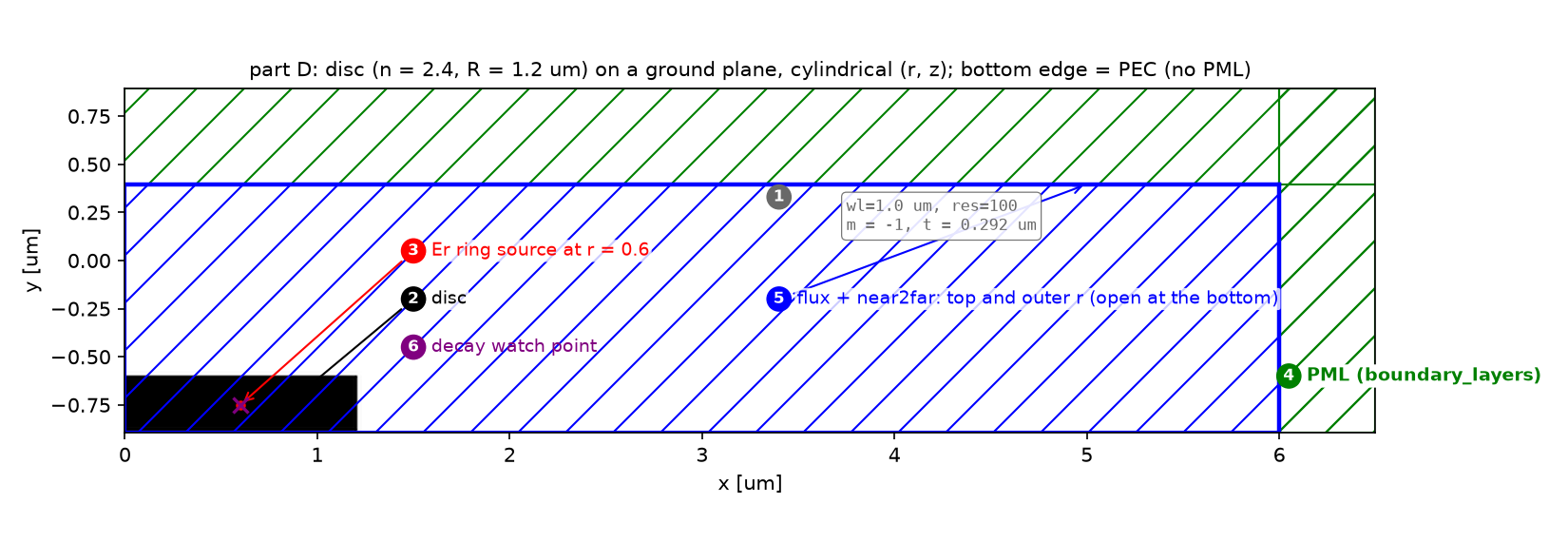
plot2D는 cylindrical 셀에서도 축 이름을 x, y로 쓰므로 x가 r, y가 z다. 동그라미 숫자는 §4의 단계 번호다.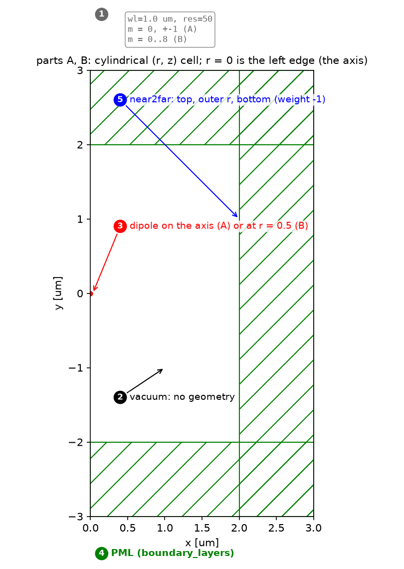
| 파라미터 | 값 | 왜 이 값인가 | 바꾸면 |
|---|---|---|---|
| A·B 셀 | r 2 + PML 1, z 4 + PML 2 | 공식 값 | near2far 면이 PML에 닿으면 안 된다 |
| A·B 해상도 | 50 | 공식 값 | Er source offset 1.5/res도 같이 바뀐다 |
| A x 쌍극자 | Er + Ep(±1j), m = ±1, r = 1.5/res | 원편광 둘의 합. r = 0의 Er은 버그(meep #2704) | m = 0으로 두면 x 쌍극자가 아니다 |
| B source | Er at r₀ = 0.5, +f와 −f 두 source | +f가 +m, −f의 켤레가 −m 항 | −f를 빼면 −m 항이 없다 |
| B 종료 기준 | m 항 power / 최대 < 10⁻⁴ | 공식 값 | 너무 느슨하면 14편의 함정(되튐) |
| C 고리 | n 3.4, R 1, w 1, PML 32, res 20 | 공식 ring-cyl.py | 셀이 r 한 줄이라 PML이 두꺼워도 싸다 |
| D 디스크 | n 2.4, R 1.2, t = 0.7λ/n, res 100 | 공식 값 | t를 바꾸면 패턴의 lobe가 바뀐다 |
| D 반지름 셀 | 6 µm(공식), 8 µm | truncation 확인 | 셀이 클수록 열린 면이 덜 잃는다 |
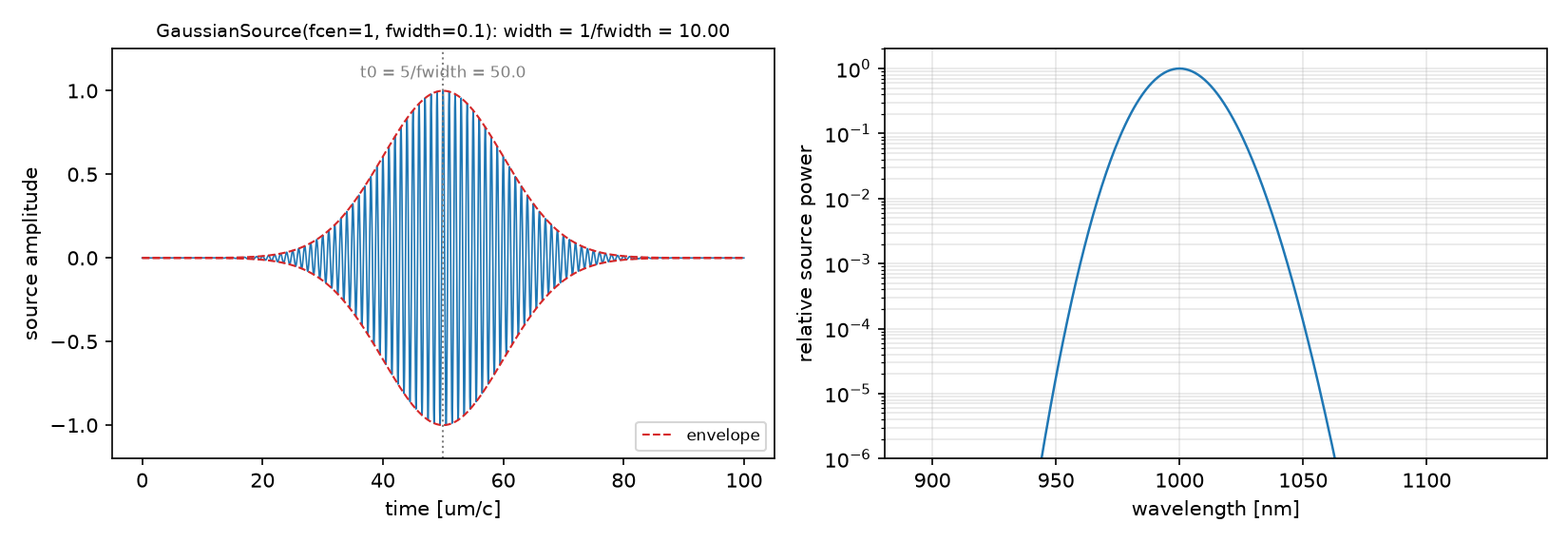
강의 노트북과의 차이: 강의 범위 밖이다. 10_sources의 노트들은 네 예제를 각각 따로 재현했다. 이 글은 한 스크립트에서 네 예제를 돌리고, B에서는 m 항을 하나 더할 때마다 패턴 오차를 재서 급수가 어떻게 수렴하는지 보이며, C에서는 12편 2D 결과와 같은 표에 올린다.
원본 코드 단계별 설명
원본 §4 · 코드 따라가기
읽는 순서: 단위·파라미터 → 재료·구조 → source → Simulation·경계 → monitor → 실행·종료 → 후처리. 이번 글의 새 요소는 ④의
dimensions=mp.CYLINDRICAL, m=과 ⑦의 m 합산이다.
① 단위와 파라미터 — 어떤 숫자를 고정하는가
WL, RES_D, PML_D = 1.0, 50, 1.0
SR_D, SZ_D = 2.0, 4.0                       # near2far box: r 0..2, z -2..2
R_FF, NPTS = 1e6 * WL, 50                   # far-field radius and polar samples
THETA = np.linspace(0, 0.5 * np.pi, NPTS)   # 0 = +z (pole), pi/2 = +r (equator), in the phi = 0 plane
POWER_DECAY = 1e-4                          # stop the m series when the last term is this small
- 무엇: 공식 값. 각도는 +z에서 잰 극각이고 φ = 0 평면의 단면이다.
- 왜: cylindrical 셀에서는 x가 r, z가 z다. y 크기는 항상 0이다.
- 틀리면: 셀을 (sr, sz, 0)처럼 3D 습관으로 쓰면 z 크기 0의 다른 문제가 된다(파트 C는 일부러 그렇게 쓴다).
② 재료와 구조 — r ≥ 0 반쪽만 그린다
mp.Block(material=mp.Medium(index=N_DISC), center=mp.Vector3(0.5 * DISC_R, 0, -0.5 * sz + 0.5 * DISC_T),
         size=mp.Vector3(DISC_R, mp.inf, DISC_T))                                         # D: a disc = a block from r 0 to R
mp.Block(center=mp.Vector3(R_IN + 0.5 * W), size=mp.Vector3(W, mp.inf, mp.inf), material=mp.Medium(index=N_RING))   # C: a ring = a block from r 1 to 2
- 무엇: 디스크는 r = 0부터 R까지의 블록, 고리는 r = 1부터 2까지의 블록이다. φ 방향 크기는
mp.inf. - 왜: (r, z) 단면에서 축 대칭 물체는 직사각형이다. 12편처럼 원기둥 두 개를 덮어쓸 필요가 없다.
- 틀리면: 블록 center를 r = 0에 두고 size를 2R로 주면 음의 r 쪽은 셀 밖이라 버려진다. 결과는 같지만 의도가 흐려진다.
③ Source — m에 따라 source가 다르다
mp.Source(gs(FREQ), component=mp.Ez, center=mp.Vector3())                              # A: z-dipole on the axis, m = 0
[mp.Source(gs(FREQ), component=mp.Er, center=mp.Vector3(r_off)),                       # A: x-dipole = Er + (+-i) Ep, run with m = +1 and m = -1
 mp.Source(gs(FREQ), component=mp.Ep, center=mp.Vector3(r_off), amplitude=1j if m == 1 else -1j)]
[mp.Source(gs(FREQ), component=mp.Er, center=mp.Vector3(R_SRC)),                       # B: off-axis, +f gives the +m term ...
 mp.Source(gs(-FREQ), component=mp.Er, center=mp.Vector3(R_SRC))]                      # ... -f gives the -m term after conjugation
- 무엇: 축 위 z 쌍극자는 Ez 하나. x 쌍극자는 m = ±1 run마다 Er과 ±i Ep의 쌍. 축 밖 점광원은 m마다 +f와 −f 두 source.
- 왜: 세 번째 줄의 요령은 $e^{-im\phi}$ 항을 따로 돌리지 않으려는 것이다. 음의 주파수 field의 켤레가 −m 항과 같아서 run 하나로 ±m을 얻는다.
- 틀리면: x 쌍극자를 m = 0의 Er 하나로 두면 축 대칭 방사(ring dipole)가 나오고 cos²θ와 전혀 다르다. 선편광은 m = 0이 아니다.
④ Simulation과 경계 — 축은 경계가 아니다
mp.Simulation(resolution=RES_D, cell_size=mp.Vector3(SR_D + PML_D, 0, SZ_D + 2 * PML_D), dimensions=mp.CYLINDRICAL, m=m,
              boundary_layers=[mp.PML(thickness=PML_D)], sources=sources, force_complex_fields=True)
boundary_layers=[mp.PML(PML_DISC, direction=mp.R), mp.PML(PML_DISC, direction=mp.Z, side=mp.High)]   # D: no PML at the bottom -> ground plane
- 무엇:
dimensions=mp.CYLINDRICAL과m. PML은 r 바깥과 z 양쪽에 붙고 축(r = 0)에는 붙지 않는다. 파트 D는 아래에 PML이 없어 그 벽이 ground plane이다. - 왜: m ≠ 0이면 field가 복소수이므로
force_complex_fields=True. 11편과 같은 규칙으로 PML을 두지 않은 셀 벽은 완전도체다. - 틀리면: 10편에서는
k_point가 벽을 주기 경계로 바꿔 거울이 사라졌다. cylindrical에는k_point가 없으므로 바닥 벽이 그대로 거울이다.
⑤ Monitor — near2far 면은 축을 닫지 않는다
mp.FluxRegion(center=mp.Vector3(0.5 * sr, 0, 0.5 * sz), size=mp.Vector3(sr, 0, 0))                  # top
mp.FluxRegion(center=mp.Vector3(sr, 0, 0), size=mp.Vector3(0, 0, sz))                                 # outer r
mp.FluxRegion(center=mp.Vector3(0.5 * sr, 0, -0.5 * sz), size=mp.Vector3(sr, 0, 0), weight=-1.0)     # bottom (A, B only)
ff = sim.get_farfield(n2f, mp.Vector3(R_FF * math.sin(th), 0, R_FF * math.cos(th)), GREENCYL_TOL)
- 무엇: A·B는 위·바깥·아래 세 조각, D는 위·바깥 두 조각(아래는 ground plane이라 둘 수 없다). far field는 φ = 0 평면의 (r, z) 점에서 구한다.
- 왜: 축은 대칭축이라 닫을 면이 없다. 회전하면 위·아래 원판과 옆 원통이 닫힌 면이 된다.
GREENCYL_TOL은 φ 방향 적분의 허용 오차다. - 틀리면: D처럼 아래가 열려 있으면 ground plane 위 바깥 r 너머의 등가 전류가 빠진다. 이것이 §5의 near–far 차이다.
⑥ 실행 — m마다 run 하나
m = 0
while True:
    sim = dipole_sim(m, src); ...; sim.run(until_after_sources=mp.stop_when_fields_decayed(20, mp.Er, mp.Vector3(R_SRC), 1e-6))
    if m > 0 and P_m / P_max < POWER_DECAY:
        break
    m += 1
- 무엇: m을 0부터 늘려 가며 run을 반복한다. 각 run은 독립이라 병렬로 돌려도 된다.
- 왜: 필요한 m의 수는 $k r_0$로 어림된다. r₀ = 0.5 µm, k = 2π/µm이면 $kr_0\approx3.1$이고, power는 m = 5 근처부터 급히 준다.
- 틀리면: 공식 코드의 종료 조건은 “처음으로 작아진 m”이다. 축에서 먼 점광원이나 구조가 있는 셀에서는 power가 줄다가 다시 커질 수 있다(10_sources Point Dipole CYL: r 3.5 µm에서 m 32의 0.5%가 m 41에서 38%로). 14편에서 다룬다.
⑦ 후처리 — field를 더하고 power를 잰다
e_tot += ep; h_tot += hp                         # +m term (exp(i m phi) = 1 at phi = 0)
if m > 0:
    e_tot += np.conj(em); h_tot += np.conj(hm)   # -m term from the negative-frequency run
pattern = radial_flux(e_tot, h_tot)              # |Re(E x H*)| on the far-field arc
P_m = total_flux(radial_flux(ep, hp))            # power of this m alone: decides when to stop
- 무엇: φ = 0에서 field를 m에 대해 더하고 Poynting으로 패턴을 만든다. 종료 판단은 m 항 하나의 power로 한다.
- 왜: 패턴은 field의 합이어야 간섭이 들어간다. 총 power는 m끼리 직교하므로 power의 합으로도 같다.
- 틀리면: 패턴을 m별 power의 합으로 만들면 간섭이 빠져 φ 의존성이 없는 평균 패턴이 나온다. x 쌍극자의 cos²θ는 간섭의 결과다.
함정: cylindrical 셀의
get_array와get_dft_array는 이 Meep 버전에서 (z, r) 순서로 돌려준다(11편). 2D처럼 전치하면 그림이 뒤집힌다. 이 글의 스크립트는 기대 크기와 비교해 방향을 맞추는orient_rz를 쓴다.
원본 결과·검증 표·오류 진단·추가 탐구
원본 §5 · 결과
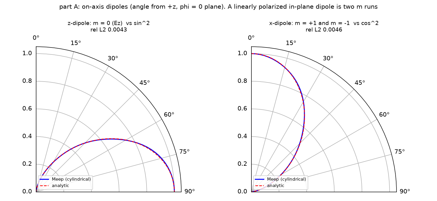
| 쌍극자 | m | 해석 패턴 | 상대 L2 |
|---|---|---|---|
| z, 축 위 | 0 | sin²θ | 0.43% |
| x, 축 위 | +1, −1 | cos²θ | 0.46% |
| m | 0 | 1 | 2 | 3 | 4 | 5 | 6 | 7 | 8 |
|---|---|---|---|---|---|---|---|---|---|
| $P_m/P_{\max}$ | 1.00 | 0.94 | 1.00 | 0.64 | 0.18 | 2.8e-2 | 2.8e-3 | 1.9e-4 | 9.5e-6 |
| 0…m 합의 패턴 오차 | 0.589 | 0.409 | 0.099 | 0.141 | 0.030 | 0.0087 | 0.0064 | 0.0064 | 0.0063 |
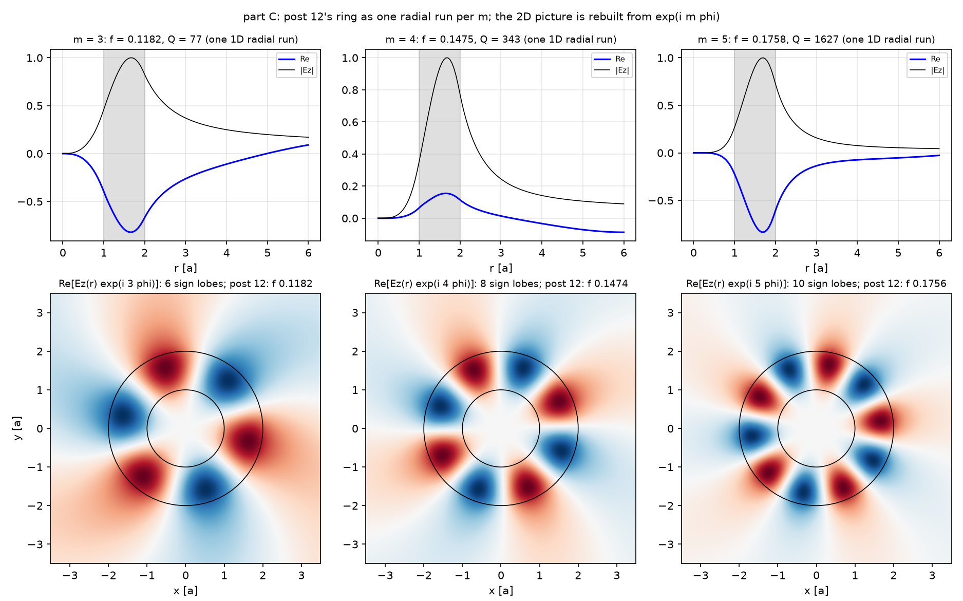
| m | f (cylindrical) | Q (cylindrical) | f (12편 2D, res 20) | Q (12편) | Δf/f |
|---|---|---|---|---|---|
| 3 | 0.11821 | 77 | 0.11818 | 79 | +0.02% |
| 4 | 0.14746 | 343 | 0.14736 | 342 | +0.07% |
| 5 | 0.17582 | 1627 | 0.17564 | 2132 | +0.10% |
| 반지름 셀 | near flux | far flux | 차이 |
|---|---|---|---|
| 6 µm (공식) | 643.65 | 595.80 | 7.43% (공식 문서 7.43%) |
| 8 µm | 643.28 | 602.05 | 6.41% |
예측과 비교
| 물리량 | 내 예측 (§2) | 시뮬레이션 | 판정 |
|---|---|---|---|
| z 쌍극자 vs sin²θ | 1% 안 | 0.43% | ✅ |
| x 쌍극자(m = ±1) vs cos²θ | 1% 안 | 0.46% | ✅ |
| r₀ = 0.5 µm에 필요한 m | 7~9 | 8 | ✅ |
| m 급수 오차 감소 | 단조 | m = 2 → 3에서 0.099 → 0.141로 증가 후 감소 | ❌ |
| ring-cyl vs 12편 주파수 | 0.2% 안 | 0.1% | ✅ |
| ring-cyl Q(m = 5) vs 12편 | 비슷 | 1627 vs 2132 | ❌ |
| 디스크 near vs far | 7% | 7.43% | ✅ |
| 셀 6 → 8 µm | 차이 감소 | 6.41% | ✅ |
여덟 예측 중 여섯이 맞았고 둘이 빗나갔다. 첫째, m 급수의 오차는 단조로 줄지 않았다. m = 0…2까지 더한 패턴(오차 0.099)이 m = 3을 더한 패턴(0.141)보다 cos²θ에 가깝다. 급수의 부분합은 해석 패턴에 한 방향으로 다가가지 않는다. m = 3 항이 아직 큰 power(0.64)를 가진 채 더해져 일시적으로 모양을 흔들고, m = 4·5가 더해진 뒤에야 맞춰진다. 그래서 “오차가 작아 보이는 중간 m에서 멈추기”는 안 되고 각 m의 power로 멈춰야 한다. 둘째, 고리의 m = 5 Q가 cylindrical에서 1627, 12편 2D(res 20)에서 2132로 30% 다르다. 그런데 12편의 2D는 res 10에서 1675, res 30에서 1610이었다. 원을 계단으로 자르지 않는 cylindrical 값은 res 10·30의 2D 값과 같은 쪽이고, 튀었던 것은 2D res 20이다. 12편에서 Q가 해상도에 비단조라고 적은 이유가 계단 경계라는 해석과 맞는다. 주파수는 세 모드 모두 0.1% 안에서 같다. 디스크의 near–far 차이는 셀 6 µm에서 공식 문서와 같은 7.43%였고 8 µm에서 6.41%로 줄었다. 열린 면이 ground plane 위 셀 바깥의 등가 전류를 잃는다는 해석과 맞는다. near flux는 셀 크기에 거의 그대로(643.65 → 643.28)라서, 줄어든 차이는 far flux 쪽이 늘어난 것이다.
수렴성
| 변수 | 값 | 결과 | 비고 |
|---|---|---|---|
| B: 포함한 m | 0…4 / 0…5 / 0…8 | 오차 0.030 / 0.0087 / 0.0063 | m = 6 이후 오차는 해상도가 정한다 |
| C: 좌표계 | 2D Cartesian(12편, res 10/20/30) vs cylindrical(res 20) | Q(m = 5) 1675/2132/1610 vs 1627 | 계단 경계가 없는 cylindrical이 res 10·30 쪽과 같다 |
| D: 반지름 셀 | 6 / 8 µm | 7.43% / 6.41% | 차이가 셀 크기를 따라가면 truncation |
주장할 수 있는 것 / 없는 것
- 할 수 있는 것: 진공에서 축 위 쌍극자의 패턴은 m = 0(z) 또는 m = ±1(x)로 0.5% 안에서 맞는다. 축에서 0.5 µm 떨어진 x 쌍극자는 m = 0…8의 합으로 0.6% 안에서 맞는다. 12편 고리의 주파수는 cylindrical 좌표와 2D Cartesian이 0.1% 안에서 같다. ground plane 위 디스크의 near–far 차이는 반지름 셀을 키우면 줄어드는 truncation이다.
- 할 수 없는 것: 축에서 먼 점광원이나 구조가 있는 셀에서 “power가 처음 10⁻⁴ 아래로 내려간 m”이 급수의 끝이라는 것(14편의 반례). 디스크의 진짜 far-field 총 power(열린 면 때문에 모른다). 2D Cartesian의 Q가 해상도마다 다른 이유를 staircase 하나로 확정하는 것(이 글은 일치하는 쪽을 보였을 뿐이다).
원본 §6 · 흔한 실수
| 증상 | 원인 | 고치는 법 |
|---|---|---|
| x 쌍극자 패턴이 축 대칭 | m = 0의 Er 하나로 둠 | m = +1과 −1, 각각 Er + (±i)Ep |
| Er source에서 field가 발산 | r = 0에 정확히 둠(meep #2704) | 1.5/res만큼 비킨다 |
| m을 다 더해도 오차 30% | −m 항(−f 켤레)을 빼먹음 | m > 0에서 conj(minus field)를 더한다 |
| 패턴에 간섭이 없음 | m별 power를 더함 | 패턴은 field를 더하고, power는 종료 판단에만 |
| 2D 그림이 뒤집힘 | cylindrical 배열은 (z, r) | 기대 크기로 방향 확인 |
| 디스크 near·far가 7% 다름 | 열린 near2far 면 | 셀을 키워 차이가 주는지 확인 |
| 바닥 거울이 사라짐 | 아래에도 PML | ground plane 쪽은 PML 없이 |
원본 §7 · 직접 해보기
| 바꿀 것 | 예상 변화 | 확인할 수치 |
|---|---|---|
| B의 r₀ 0.5 → 1.5 µm | 필요한 m이 약 3배(kr₀에 비례) | 마지막 m, 각 m power의 되튐 |
| B를 y 쌍극자(Ep)로 | 패턴이 상수 | 상대 L2 vs 1 |
| C에서 m = 2 | 대역 0.10~0.20 밖, 낮은 Q | Harminv 결과 |
| D의 반지름 셀 12 µm | 차이가 더 준다 | near·far 차이 |
| D의 디스크 두께 0.7λ/n → 0.5λ/n | lobe가 바뀐다 | 패턴 |
code/cylindrical_dipole.py 전체 (클릭하여 펼치기)
"""Meep Example 13 - Computing 3D with rotational symmetry: cylindrical coordinates and the m series.

Post 12's ring was a 2D cross-section. A real disc or ring is a body of revolution, and Meep's
dimensions=mp.CYLINDRICAL solves it as one 2D (r, z) run per azimuthal order m, with fields ~ exp(i m phi).
  A. On-axis dipoles in vacuum (official dipole_in_vacuum_cyl_on_axis.py): a z-dipole is m = 0 (Ez);
     an x-dipole is NOT m = 0 but the sum of m = +1 and m = -1 (Er + i Ep, Er - i Ep). Far-field
     patterns vs the analytic cos^2(theta) and sin^2(theta).
  B. An off-axis x-dipole at r = 0.5 um (official dipole_in_vacuum_cyl_off_axis.py): a point away from
     the axis is a Fourier series over m = 0, 1, 2, ... The series is summed until the power of the last
     m drops below 1e-4 of the largest; the pattern is checked after every added m.
  C. The ring of post 12 in cylindrical coordinates (official ring-cyl.py): one 1D radial run per m.
     Frequencies and Q compared with post 12's 2D Cartesian values; the m = 3 field rebuilt in the
     x-y plane from Ez(r) exp(i m phi).
  D. A dielectric disc on a ground plane (official disc_radiation_pattern.py): a ring source (m = -1),
     near flux vs far-field flux; the 7 % gap comes from the open near2far surface, checked by
     enlarging the radial cell.
MPI-safe: collective calls on every rank, figures on the master only.

Run:  mpirun -np 4 python cylindrical_dipole.py     (~6 min)
Out:  00_source.png, 01_layout.png, 02_layout_dipole.png, 03_on_axis.png, 04_off_axis.png, 05_ring_cyl.png,
      06_disc.png, 07_anim_m3.gif, result.json   (-> ../assets/13/)
"""
import cmath
import json
import math
import os
import sys
import time

import numpy as np
import matplotlib
matplotlib.use("Agg")
import matplotlib.pyplot as plt
from matplotlib import animation
import meep as mp

sys.path.insert(0, os.path.dirname(os.path.abspath(__file__)))
from blogfig import Label, annotated_layout, source_figure   # noqa: E402

HERE = os.path.dirname(os.path.abspath(__file__))
OUT = os.path.join(HERE, "..", "assets", "13")
os.makedirs(OUT, exist_ok=True)
MASTER = mp.am_master()
t_all = time.time()


def say(*a):
    if MASTER:
        print(*a, flush=True)


def rel_l2(a, b):
    return float(np.linalg.norm(np.asarray(a) - np.asarray(b)) / np.linalg.norm(np.asarray(b)))


def orient_rz(arr, nr):
    """Cylindrical get_array/get_dft_array return (z, r) in this Meep version; return (r, z) whatever the order."""
    arr = np.asarray(arr)
    if arr.ndim == 2 and abs(arr.shape[1] - nr) < abs(arr.shape[0] - nr):
        return arr.T
    return arr


# ---------------------------------------------------------------- (1) parameters shared by A and B (official values, um)
WL = 1.0
FREQ = 1 / WL
RES_D = 50
PML_D = 1.0
SR_D, SZ_D = 2.0, 4.0                       # near2far box: r 0..2, z -2..2
R_FF = 1e6 * WL
NPTS = 50
THETA = np.linspace(0, 0.5 * np.pi, NPTS)   # 0 = +z (pole), pi/2 = +r (equator), in the phi = 0 plane
GREENCYL_TOL = 1e-6
POWER_DECAY = 1e-4


def n2f_regions(sr, sz):
    return [mp.FluxRegion(center=mp.Vector3(0.5 * sr, 0, 0.5 * sz), size=mp.Vector3(sr, 0, 0)),
            mp.FluxRegion(center=mp.Vector3(sr, 0, 0), size=mp.Vector3(0, 0, sz)),
            mp.FluxRegion(center=mp.Vector3(0.5 * sr, 0, -0.5 * sz), size=mp.Vector3(sr, 0, 0), weight=-1.0)]


def farfields(sim, n2f, tol=GREENCYL_TOL, theta=THETA, r_ff=R_FF):
    e = np.zeros((len(theta), 3), complex); h = np.zeros((len(theta), 3), complex)
    for n, th in enumerate(theta):
        ff = sim.get_farfield(n2f, mp.Vector3(r_ff * math.sin(th), 0, r_ff * math.cos(th)), tol)
        e[n] = ff[:3]; h[n] = ff[3:]
    return e, h


def radial_flux(e, h):
    fx = np.real(e[:, 1] * np.conj(h[:, 2]) - e[:, 2] * np.conj(h[:, 1]))
    fz = np.real(e[:, 0] * np.conj(h[:, 1]) - e[:, 1] * np.conj(h[:, 0]))
    return np.sqrt(fx ** 2 + fz ** 2)


def total_flux(pattern, theta=THETA, r_ff=R_FF):
    return float(2 * np.pi * r_ff ** 2 * np.trapezoid(pattern * np.sin(theta), theta))


def dipole_sim(m, sources):
    return mp.Simulation(resolution=RES_D, cell_size=mp.Vector3(SR_D + PML_D, 0, SZ_D + 2 * PML_D), dimensions=mp.CYLINDRICAL, m=m,
                         boundary_layers=[mp.PML(thickness=PML_D)], sources=sources, force_complex_fields=True)


# ================================================================ A. on-axis dipoles
t_a = time.time()
r_off = 1.5 / RES_D                          # an Er source exactly at r = 0 hits a known bug (meep issue 2704): offset by 1.5 px
gs = lambda f: mp.GaussianSource(f, fwidth=0.1 * abs(f))
on = {}
# z-dipole: m = 0, Ez on the axis
sim = dipole_sim(0, [mp.Source(gs(FREQ), component=mp.Ez, center=mp.Vector3())])
annotated_layout(sim, os.path.join(OUT, "02_layout_dipole.png"), dpml=PML_D, figsize=(5.4, 7.6), axis_step=1.0, unit="um",
                 title="parts A, B: cylindrical (r, z) cell; r = 0 is the left edge (the axis)",
                 params_text=f"wl={WL} um, res={RES_D}\nm = 0, +-1 (A)\nm = 0..8 (B)", params_xy=(0.15, 3.75), pml_xy=(0.15, -3.5), decay_point=None,
                 labels=[Label("dipole on the axis (A) or at r = 0.5 (B)", (0.03, 0.0), (0.4, 0.9), step=3, color="red"),
                         Label("near2far: top, outer r, bottom (weight -1)", (2.0, 1.0), (0.4, 2.6), step=5, color="blue"),
                         Label("vacuum: no geometry", (1.0, -1.0), (0.4, -1.4), step=2, color="black")])
n2f = sim.add_near2far(FREQ, 0, 1, *n2f_regions(SR_D, SZ_D))
sim.run(until_after_sources=mp.stop_when_fields_decayed(20, mp.Ez, mp.Vector3(), 1e-6))
on["z"] = farfields(sim, n2f); sim.reset_meep()
# x-dipole: m = +1 and m = -1, each Er + (+-i) Ep, combined with weight 1/2 and exp(+-i phi) at phi = 0
ex = np.zeros((NPTS, 3), complex); hx = np.zeros((NPTS, 3), complex)
for m in (+1, -1):
    src = [mp.Source(gs(FREQ), component=mp.Er, center=mp.Vector3(r_off)),
           mp.Source(gs(FREQ), component=mp.Ep, center=mp.Vector3(r_off), amplitude=1j if m == 1 else -1j)]
    sim = dipole_sim(m, src)
    n2f = sim.add_near2far(FREQ, 0, 1, *n2f_regions(SR_D, SZ_D))
    sim.run(until_after_sources=mp.stop_when_fields_decayed(20, mp.Er, mp.Vector3(r_off), 1e-6))
    e, h = farfields(sim, n2f); sim.reset_meep()
    ex += 0.5 * e; hx += 0.5 * h
on["x"] = (ex, hx)
pat_on = {k: radial_flux(*v) for k, v in on.items()}
an_on = {"x": np.cos(THETA) ** 2, "z": np.sin(THETA) ** 2}
err_on = {k: rel_l2(pat_on[k] / pat_on[k].max(), an_on[k]) for k in on}
say(f"A: on-axis z-dipole (m = 0) vs sin^2: rel L2 {err_on['z']:.4f}; x-dipole (m = +1 and -1) vs cos^2: {err_on['x']:.4f}; {time.time() - t_a:.0f} s")
if MASTER:
    source_figure(FREQ, 0.1 * FREQ, os.path.join(OUT, "00_source.png"), wl_scale=1000.0, wl_unit="nm", time_unit="um/c")

# ================================================================ B. off-axis x-dipole: the m series
t_b = time.time()
R_SRC = 0.5
e_tot = np.zeros((NPTS, 3), complex); h_tot = np.zeros((NPTS, 3), complex)
m_flux, m_err, flux_max = [], [], 0.0
m = 0
while True:
    src = [mp.Source(gs(FREQ), component=mp.Er, center=mp.Vector3(R_SRC)),
           mp.Source(gs(-FREQ), component=mp.Er, center=mp.Vector3(R_SRC))]          # +f gives the +m term, -f the -m term (conjugated)
    sim = dipole_sim(m, src)
    n2p = sim.add_near2far(FREQ, 0, 1, *n2f_regions(SR_D, SZ_D))
    n2m = sim.add_near2far(-FREQ, 0, 1, *n2f_regions(SR_D, SZ_D))
    sim.run(until_after_sources=mp.stop_when_fields_decayed(20, mp.Er, mp.Vector3(R_SRC), 1e-6))
    ep, hp = farfields(sim, n2p); em, hm = farfields(sim, n2m); sim.reset_meep()
    e_tot += ep; h_tot += hp                                   # exp(i m phi) = 1 at phi = 0
    if m > 0:
        e_tot += np.conj(em); h_tot += np.conj(hm)
    fl = total_flux(radial_flux(ep, hp))
    flux_max = max(flux_max, fl)
    p = radial_flux(e_tot, h_tot)
    m_flux.append(fl); m_err.append(rel_l2(p / p.max(), np.cos(THETA) ** 2))
    say(f"B: m = {m}: power of this m / max = {fl / flux_max:.2e}; pattern error after summing 0..{m}: {m_err[-1]:.4f}")
    if m > 0 and fl / flux_max < POWER_DECAY:
        break
    m += 1
pat_off = radial_flux(e_tot, h_tot)
say(f"B: off-axis x-dipole at r = {R_SRC}: stopped at m = {m}; final rel L2 vs cos^2 {m_err[-1]:.4f}; {time.time() - t_b:.0f} s")

# ================================================================ C. post 12's ring in cylindrical coordinates
t_c = time.time()
N_RING, W, R_IN, PAD, DPML_R = 3.4, 1.0, 1.0, 4.0, 32.0
SR_R = R_IN + W + PAD + DPML_R
RES_R = 20
FC, DFC = 0.15, 0.1
POST12 = {3: (0.11818, 79), 4: (0.14736, 342), 5: (0.17564, 2132)}     # 2D Cartesian, res 20 (post 12)
ring = {}


def ring_sim(m, f, df):
    return mp.Simulation(cell_size=mp.Vector3(SR_R, 0, 0), resolution=RES_R, dimensions=mp.CYLINDRICAL, m=m, boundary_layers=[mp.PML(DPML_R)],
                         geometry=[mp.Block(center=mp.Vector3(R_IN + 0.5 * W), size=mp.Vector3(W, mp.inf, mp.inf), material=mp.Medium(index=N_RING))],
                         sources=[mp.Source(mp.GaussianSource(f, fwidth=df), component=mp.Ez, center=mp.Vector3(R_IN + 0.1))])


for mm in (3, 4, 5):
    sim = ring_sim(mm, FC, DFC)
    hv = mp.Harminv(mp.Ez, mp.Vector3(R_IN + 0.1), FC, DFC)
    sim.run(mp.after_sources(hv), until_after_sources=200)
    modes = [md for md in hv.modes if md.Q > 0 and FC - 0.5 * DFC < md.freq < FC + 0.5 * DFC]
    md = max(modes, key=lambda x: abs(x.amp)); sim.reset_meep()
    f, Q = float(md.freq), float(md.Q)
    sim = ring_sim(mm, f, 0.01)
    dft = sim.add_dft_fields([mp.Ez], f, 0, 1, center=mp.Vector3(0.5 * (R_IN + W + PAD)), size=mp.Vector3(R_IN + W + PAD))
    sim.run(until_after_sources=mp.stop_when_fields_decayed(50, mp.Ez, mp.Vector3(R_IN + 0.1), 1e-6))
    ezr = np.squeeze(sim.get_dft_array(dft, mp.Ez, 0)); sim.reset_meep()
    ring[mm] = {"f": f, "Q": Q, "ez_r": ezr}
    say(f"C: m = {mm}: cylindrical f {f:.5f} Q {Q:.0f} | post 12 (2D, res 20): f {POST12[mm][0]:.5f} Q {POST12[mm][1]} -> df/f {(f - POST12[mm][0]) / POST12[mm][0]:+.2e}")
say(f"C done in {time.time() - t_c:.0f} s")

# ================================================================ D. disc on a ground plane, near vs far flux
t_d = time.time()
RES_DISC, PML_DISC, AIR = 100, 0.5, 1.0
DISC_R, N_DISC = 1.2, 2.4
DISC_T = 0.7 * WL / N_DISC
NPOL = 100
THETA_D = np.linspace(0, 0.5 * np.pi, NPOL)
disc = {}
for cell_r in (6.0, 8.0):
    sr = cell_r + PML_DISC; sz = DISC_T + AIR + PML_DISC
    src_pt = mp.Vector3(0.5 * DISC_R, 0, -0.5 * sz + 0.5 * DISC_T)
    sim = mp.Simulation(resolution=RES_DISC, cell_size=mp.Vector3(sr, 0, sz), dimensions=mp.CYLINDRICAL, m=-1,
                        boundary_layers=[mp.PML(PML_DISC, direction=mp.R), mp.PML(PML_DISC, direction=mp.Z, side=mp.High)],   # no PML at the bottom: PEC ground plane
                        sources=[mp.Source(mp.GaussianSource(FREQ, fwidth=0.1 * FREQ), component=mp.Er, center=src_pt)],
                        geometry=[mp.Block(material=mp.Medium(index=N_DISC), center=mp.Vector3(0.5 * DISC_R, 0, -0.5 * sz + 0.5 * DISC_T), size=mp.Vector3(DISC_R, mp.inf, DISC_T))])
    regs = [mp.FluxRegion(center=mp.Vector3(0.5 * cell_r, 0, 0.5 * sz - PML_DISC), size=mp.Vector3(cell_r, 0, 0)),
            mp.FluxRegion(center=mp.Vector3(cell_r, 0, 0.5 * sz - PML_DISC - 0.5 * (AIR + DISC_T)), size=mp.Vector3(0, 0, AIR + DISC_T))]
    flux = sim.add_flux(FREQ, 0, 1, *regs)
    n2f = sim.add_near2far(FREQ, 0, 1, *regs)
    dft = None
    if cell_r == 6.0:
        dft = sim.add_dft_fields([mp.Er], FREQ, 0, 1, center=mp.Vector3(0.5 * cell_r, 0, -0.5 * PML_DISC), size=mp.Vector3(cell_r, 0, sz - PML_DISC))
        annotated_layout(sim, os.path.join(OUT, "01_layout.png"), dpml=PML_DISC, figsize=(11, 3.8), axis_step=1.0, unit="um",
                         title="part D: disc (n = 2.4, R = 1.2 um) on a ground plane, cylindrical (r, z); bottom edge = PEC (no PML)",
                         params_text=f"wl={WL} um, res={RES_DISC}\nm = -1, t = {DISC_T:.3f} um", params_xy=(3.4, 0.33), pml_xy=(6.05, -0.6),
                         decay_point=(src_pt.x, src_pt.z), decay_text_xy=(1.5, -0.45),
                         labels=[Label("disc", (0.9, src_pt.z + 0.05), (1.5, -0.2), step=2, color="black"),
                                 Label("Er ring source at r = 0.6", (src_pt.x, src_pt.z), (1.5, 0.05), step=3, color="red"),
                                 Label("flux + near2far: top and outer r (open at the bottom)", (5.0, 0.5 * sz - PML_DISC), (3.4, -0.2), step=5, color="blue")])
    sim.run(until_after_sources=mp.stop_when_fields_decayed(50, mp.Er, src_pt, 1e-8))
    f_near = float(mp.get_fluxes(flux)[0])
    e, h = farfields(sim, n2f, tol=1e-8, theta=THETA_D)
    pat = radial_flux(e, h)
    f_far = total_flux(pat, theta=THETA_D)
    er = orient_rz(sim.get_dft_array(dft, mp.Er, 0), int(round(cell_r * RES_DISC))) if dft is not None else None
    sim.reset_meep()
    disc[cell_r] = {"near": f_near, "far": f_far, "gap": abs(f_near - f_far) / f_near, "pattern": pat, "er": er, "sz": sz}
    say(f"D: cell r {cell_r}: near flux {f_near:.4f}, far flux {f_far:.4f}, gap {100 * disc[cell_r]['gap']:.2f} %")
say(f"D done in {time.time() - t_d:.0f} s")

# ================================================================ figures (master only)
if MASTER:
    # A
    fig, ax = plt.subplots(1, 2, figsize=(10, 4.6), subplot_kw={"projection": "polar"})
    for a, k, lab in ((ax[0], "z", "z-dipole: m = 0 (Ez)  vs sin^2"), (ax[1], "x", "x-dipole: m = +1 and m = -1  vs cos^2")):
        a.plot(THETA, pat_on[k] / pat_on[k].max(), "b-", lw=1.6, label="Meep (cylindrical)")
        a.plot(THETA, an_on[k], "r--", lw=1.2, label="analytic")
        a.set_theta_zero_location("N"); a.set_theta_direction(-1); a.set_thetamin(0); a.set_thetamax(90); a.set_rmax(1.05)
        a.set_title(f"{lab}\nrel L2 {err_on[k]:.4f}", fontsize=9); a.legend(fontsize=7, loc="lower left")
    fig.suptitle("part A: on-axis dipoles (angle from +z, phi = 0 plane). A linearly polarized in-plane dipole is two m runs", fontsize=10)
    fig.tight_layout(); fig.savefig(os.path.join(OUT, "03_on_axis.png"), dpi=150); plt.close(fig)
    # B
    fig = plt.figure(figsize=(13, 4.4))
    ax = fig.add_subplot(1, 3, 1)
    ms = np.arange(len(m_flux))
    ax.semilogy(ms, np.array(m_flux) / max(m_flux), "o-", color="tab:blue"); ax.axhline(POWER_DECAY, color="crimson", ls="--", lw=1, label="stop: 1e-4 of the max")
    ax.set_xlabel("azimuthal order m"); ax.set_ylabel("far-field power of the m term / max"); ax.set_title(f"dipole at r = {R_SRC} um: how much each m radiates", fontsize=9); ax.grid(alpha=0.3, which="both"); ax.legend(fontsize=8)
    ax = fig.add_subplot(1, 3, 2)
    ax.semilogy(ms, m_err, "s-", color="tab:green"); ax.set_xlabel("m included up to"); ax.set_ylabel("rel L2 of the summed pattern vs cos^2"); ax.set_title("the pattern converges as m terms are added", fontsize=9); ax.grid(alpha=0.3, which="both")
    ax = fig.add_subplot(1, 3, 3, projection="polar")
    ax.plot(THETA, pat_off / pat_off.max(), "b-", lw=1.6, label=f"Meep, m = 0..{m}"); ax.plot(THETA, np.cos(THETA) ** 2, "r--", lw=1.2, label="cos^2")
    ax.set_theta_zero_location("N"); ax.set_theta_direction(-1); ax.set_thetamin(0); ax.set_thetamax(90); ax.set_rmax(1.05); ax.legend(fontsize=7, loc="lower left")
    ax.set_title(f"off-axis x-dipole: rel L2 {m_err[-1]:.4f}", fontsize=9)
    fig.suptitle("part B: a point away from the axis is a Fourier series over m; each m is one 2D (r, z) run", fontsize=10)
    fig.tight_layout(); fig.savefig(os.path.join(OUT, "04_off_axis.png"), dpi=150); plt.close(fig)
    # C: Ez(r) and the x-y reconstruction for m = 3, 4, 5
    rr = np.linspace(0, R_IN + W + PAD, len(ring[3]["ez_r"]))
    L = R_IN + W + 1.5
    xg = np.linspace(-L, L, 301); X, Y = np.meshgrid(xg, xg, indexing="ij"); RG = np.hypot(X, Y); PH = np.arctan2(Y, X)
    fig, ax = plt.subplots(2, 3, figsize=(12.5, 7.8), gridspec_kw={"height_ratios": [1, 1.5]})
    for k, mm in enumerate((3, 4, 5)):
        d = ring[mm]; ez = d["ez_r"] / np.max(np.abs(d["ez_r"]))
        ax[0, k].plot(rr, np.real(ez), "b-", label="Re"); ax[0, k].plot(rr, np.abs(ez), "k-", lw=0.8, label="|Ez|")
        ax[0, k].axvspan(R_IN, R_IN + W, color="gray", alpha=0.25); ax[0, k].set_xlabel("r [a]"); ax[0, k].set_title(f"m = {mm}: f = {d['f']:.4f}, Q = {d['Q']:.0f} (one 1D radial run)", fontsize=9)
        ax[0, k].grid(alpha=0.3); ax[0, k].legend(fontsize=7)
        field = np.real(np.interp(RG, rr, np.real(ez)) * np.cos(mm * PH) - np.interp(RG, rr, np.imag(ez)) * np.sin(mm * PH))
        field[RG > rr[-1]] = 0
        lim = np.max(np.abs(field))
        ax[1, k].imshow(field.T, extent=[-L, L, -L, L], origin="lower", cmap="RdBu", vmin=-lim, vmax=lim, aspect="equal")
        for rc in (R_IN, R_IN + W):
            ax[1, k].add_patch(plt.Circle((0, 0), rc, fill=False, color="k", lw=0.8))
        ax[1, k].set_title(f"Re[Ez(r) exp(i {mm} phi)]: {2 * mm} sign lobes; post 12: f {POST12[mm][0]:.4f}", fontsize=9); ax[1, k].set_xlabel("x [a]")
    ax[1, 0].set_ylabel("y [a]")
    fig.suptitle("part C: post 12's ring as one radial run per m; the 2D picture is rebuilt from exp(i m phi)", fontsize=10)
    fig.tight_layout(); fig.savefig(os.path.join(OUT, "05_ring_cyl.png"), dpi=150); plt.close(fig)
    # D
    fig = plt.figure(figsize=(13.5, 4.4))
    ax = fig.add_subplot(1, 3, 1, projection="polar")
    for cr, c in ((6.0, "tab:blue"), (8.0, "tab:orange")):
        p = disc[cr]["pattern"]; ax.plot(THETA_D, p / disc[6.0]["pattern"].max(), "-", color=c, lw=1.4, label=f"cell r {cr:.0f} um")
    ax.set_theta_zero_location("N"); ax.set_theta_direction(-1); ax.set_thetamin(0); ax.set_thetamax(90); ax.legend(fontsize=7, loc="lower left")
    ax.set_title("disc on a ground plane: far-field pattern", fontsize=9)
    ax = fig.add_subplot(1, 3, 2)
    idx = np.arange(2)
    ax.bar(idx - 0.2, [disc[c]["near"] for c in (6.0, 8.0)], width=0.4, color="tab:gray", label="near flux (monitor)")
    ax.bar(idx + 0.2, [disc[c]["far"] for c in (6.0, 8.0)], width=0.4, color="tab:blue", label="far flux (hemisphere integral)")
    for k, c in enumerate((6.0, 8.0)):
        ax.text(k, max(disc[c]["near"], disc[c]["far"]) * 1.02, f"gap {100 * disc[c]['gap']:.2f} %", ha="center", fontsize=8)
    ax.set_xticks(idx); ax.set_xticklabels(["cell r 6 um", "cell r 8 um"]); ax.set_ylabel("power (a.u.)"); ax.set_title("the open near2far surface misses currents on the ground plane", fontsize=9); ax.legend(fontsize=7, loc="lower right")
    ax = fig.add_subplot(1, 3, 3)
    er = disc[6.0]["er"]; sz = disc[6.0]["sz"]
    ax.imshow(np.log10(np.abs(er) + 1e-12).T, extent=[0, 6.0, -0.5 * sz, 0.5 * sz - PML_DISC], origin="lower", cmap="inferno", aspect="auto")
    ax.add_patch(plt.Rectangle((0, -0.5 * sz), DISC_R, DISC_T, fill=False, color="w", lw=1))
    ax.set_xlabel("r [um]"); ax.set_ylabel("z [um]"); ax.set_title("log10 |Er| at 1 um (r, z plane)", fontsize=9)
    fig.suptitle("part D: near vs far flux; the gap shrinks when the radial cell grows", fontsize=10)
    fig.tight_layout(); fig.savefig(os.path.join(OUT, "06_disc.png"), dpi=150); plt.close(fig)
    # GIF: m = 3 mode rotating: Re[Ez(r) exp(i (3 phi - w t))]
    d = ring[3]; ez = d["ez_r"] / np.max(np.abs(d["ez_r"]))
    Er_ = np.interp(RG, rr, np.real(ez)); Ei_ = np.interp(RG, rr, np.imag(ez)); amp = np.where(RG > rr[-1], 0, 1)
    fig_g, ax_g = plt.subplots(figsize=(4.8, 4.4))
    im = ax_g.imshow(np.zeros_like(RG).T, extent=[-L, L, -L, L], origin="lower", cmap="RdBu", vmin=-1, vmax=1, aspect="equal")
    for rc in (R_IN, R_IN + W):
        ax_g.add_patch(plt.Circle((0, 0), rc, fill=False, color="k", lw=0.8))
    ax_g.set_xlabel("x [a]"); ax_g.set_ylabel("y [a]"); ttl = ax_g.set_title("", fontsize=9); fig_g.tight_layout()
    NF = 36

    def upd(i):
        wt = 2 * np.pi * i / NF
        fld = amp * (Er_ * np.cos(3 * PH - wt) - Ei_ * np.sin(3 * PH - wt))
        im.set_data((fld / np.max(np.abs(fld))).T); ttl.set_text(f"m = 3 mode, Re[Ez(r) exp(i(3 phi - wt))], wt = {np.degrees(wt):.0f} deg")
        return im, ttl

    animation.FuncAnimation(fig_g, upd, frames=NF, blit=False).save(os.path.join(OUT, "07_anim_m3.gif"), writer=animation.PillowWriter(fps=12), dpi=75)
    plt.close(fig_g)
    with open(os.path.join(OUT, "result.json"), "w") as f_:
        json.dump({"A": {"err_z": err_on["z"], "err_x": err_on["x"]},
                   "B": {"r_src": R_SRC, "m_last": m, "m_flux_rel": (np.array(m_flux) / max(m_flux)).tolist(), "m_err": m_err},
                   "C": {str(k): {"f": v["f"], "Q": v["Q"], "post12_f": POST12[k][0], "post12_Q": POST12[k][1]} for k, v in ring.items()},
                   "D": {str(k): {"near": v["near"], "far": v["far"], "gap": v["gap"]} for k, v in disc.items()},
                   "wall_s_total": time.time() - t_all, "np": mp.count_processors(), "meep": mp.__version__}, f_, indent=2)
say(f"total {time.time() - t_all:.0f} s on {mp.count_processors()} process(es)")
원본 실행 기록과 재현 환경
§4의 발췌 코드와 달리 전체 코드에는 두 layout 그림, m 급수 수렴 그림, 고리의 x–y 복원, 디스크 field, GIF, result.json 기록이 들어 있다. MPI로 돌릴 수 있게 collective 호출(run, get_farfield, get_dft_array)은 모든 rank에서, 그림 저장은 master에서만 한다. 전체 코드와 helper: https://github.com/jin-castle/meep-examples/blob/main/code.
실행 결과 (2026-10-23 실행, mpirun -np 4):
A: on-axis z-dipole (m = 0) vs sin^2: rel L2 0.0043; x-dipole (m = +1 and -1) vs cos^2: 0.0046; 53 s
B: m = 0: power of this m / max = 1.00e+00; pattern error after summing 0..0: 0.5890
B: m = 1: power of this m / max = 9.36e-01; pattern error after summing 0..1: 0.4094
B: m = 2: power of this m / max = 1.00e+00; pattern error after summing 0..2: 0.0987
B: m = 3: power of this m / max = 6.36e-01; pattern error after summing 0..3: 0.1405
B: m = 4: power of this m / max = 1.80e-01; pattern error after summing 0..4: 0.0298
B: m = 5: power of this m / max = 2.79e-02; pattern error after summing 0..5: 0.0087
B: m = 6: power of this m / max = 2.78e-03; pattern error after summing 0..6: 0.0064
B: m = 7: power of this m / max = 1.90e-04; pattern error after summing 0..7: 0.0064
B: m = 8: power of this m / max = 9.49e-06; pattern error after summing 0..8: 0.0063
B: off-axis x-dipole at r = 0.5: stopped at m = 8; final rel L2 vs cos^2 0.0063; 139 s
C: m = 3: cylindrical f 0.11821 Q 77 | post 12 (2D, res 20): f 0.11818 Q 79 -> df/f +2.30e-04
C: m = 4: cylindrical f 0.14746 Q 343 | post 12 (2D, res 20): f 0.14736 Q 342 -> df/f +6.62e-04
C: m = 5: cylindrical f 0.17582 Q 1627 | post 12 (2D, res 20): f 0.17564 Q 2132 -> df/f +1.02e-03
D: cell r 6.0: near flux 643.6506, far flux 595.8024, gap 7.43 %
D: cell r 8.0: near flux 643.2784, far flux 602.0512, gap 6.41 %
total 457 s on 4 process(es)
재현 환경: meep 1.33.0 (MPI) · Python 3.11 · conda install -c conda-forge pymeep=*=mpi_mpich_* · 실행 mpirun -np 4 python cylindrical_dipole.py (약 7.6 min (mpirun -np 4))
공식 문서와 다음 글
- Cylindrical coordinates 튜토리얼 · antenna in cylindrical coordinates · disc in cylindrical coordinates
- 스크립트: dipole_in_vacuum_cyl_on_axis.py · dipole_in_vacuum_cyl_off_axis.py · ring-cyl.py · disc_radiation_pattern.py · meep issue 2704 (Er at r = 0)
- 이전 글: 12 · 빛을 가두는 고리 · near2far와 거울: 10 · 점광원의 3D 방사 패턴 · 다음 글: 14 · 박막 속 점광원, 공기로 나오는 몫