MEEP EXAMPLES 11
두 거울 사이에서 빛의 양은 어떻게 달라질까?
같은 쌍극자의 LDOS를 거울 유무에 따라 비교합니다. Purcell 인자, 모드 cutoff, 높은 Q에서의 실행 시간 한계를 읽습니다.
이 글을 읽고 나면
- 같은 source의 cavity·bulk 비율로 Purcell 인자를 구한다.
- 평면 cavity의 cutoff와 두 좌표계의 결과를 해석한다.
- 2D 상자의 Q·LDOS와 미수렴 결과를 구별한다.
먼저 알면 좋은 것 01편 점원 · 10편 PEC와 image dipole
1. 먼저 보기: 거울은 빛의 양도 바꿀까?
10편에서는 거울 하나가 빛이 나가는 방향을 바꿨습니다. 이번에는 같은 쌍극자를 두 거울 사이에 놓았을 때 방출 power가 얼마나 달라지는지 봅니다. source 위치에서 잰 LDOS를 거울 없는 bulk의 LDOS로 나눈 값이 Purcell 인자입니다.
두 실험의 물리량을 구별하세요. 파트 A는 손실 없는 평면 거울 사이에서 bulk로 정규화한 Purcell 인자를 계산합니다. 파트 B는 구멍이 있는 2D PEC 상자의 raw LDOS와 Q/V 근사를 비교합니다. 파트 B의 숫자를 검증된 3D Purcell 인자로 해석할 수 없습니다.
2. 먼저 예측하기: 거울을 두면 항상 더 밝아질까?
예측과 실제 결과 비교하기
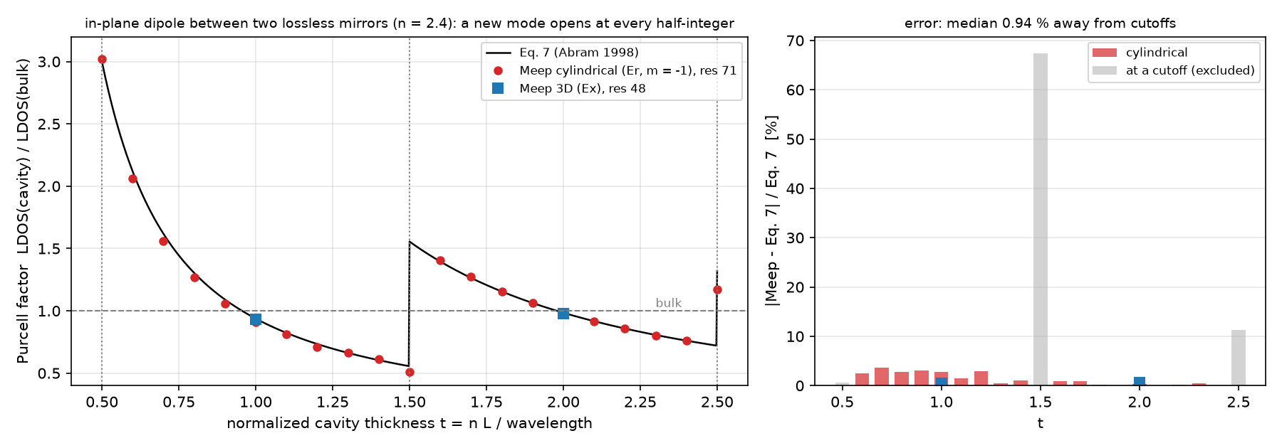
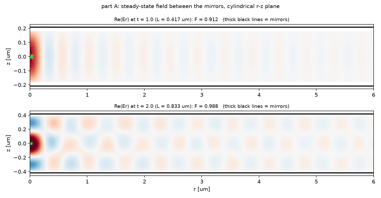
두 번째입니다. t = 1.0에서 cylindrical 계산은 0.912, 3D는 0.933, 해석식은 0.9375입니다. 모두 1보다 작습니다. 거울은 source가 결합할 수 있는 모드를 바꾸므로 방출을 강화할 수도, 억제할 수도 있습니다.
3. 원리 이해하기: 같은 source로 두 번 재는 이유
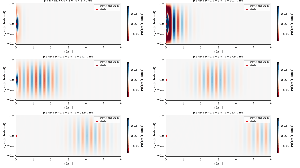
쌍극자는 자신이 만든 field와 상호작용합니다. 거울에서 돌아온 field가 source 자리의 응답을 바꾸면, 같은 진폭의 전류가 내는 power도 달라집니다. dft_ldos는 source 자리의 field와 전류의 주파수 성분으로 이 응답을 구합니다.
F_P = LDOS(cavity) / LDOS(bulk)로 나누면 같은 source·좌표계·격자 정규화의 영향을 비교에서 상쇄할 수 있습니다. cylindrical과 3D는 각각 자신의 bulk run으로 나눠야 합니다.
거울 간격은 매질 안 파장으로 환산한 t = nL/λ로 읽습니다. 이 평면 cavity와 in-plane 쌍극자에서는 t가 0.5, 1.5, 2.5를 지날 때 모드가 새로 열리며 해석식이 불연속으로 뜁니다. 이 지점이 cutoff입니다. 유한 격자와 유한 시간으로 계산한 cutoff 값을 매끈한 구간과 같은 오차 통계에 섞지 않습니다.
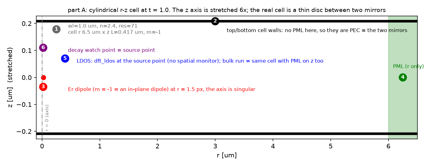
평면 cavity의 조건. 파장 1 µm, 굴절률 2.4, 손실 없는 매질·PEC 거울입니다. cylindrical은 Er와 m = −1, 3D는 Ex로 in-plane 쌍극자를 표현합니다. 거울 방향 z에는 PML을 두지 않고 옆으로 나가는 파만 흡수합니다. 손실 매질의 점광원 LDOS에 이 절차를 그대로 적용할 수는 없습니다.
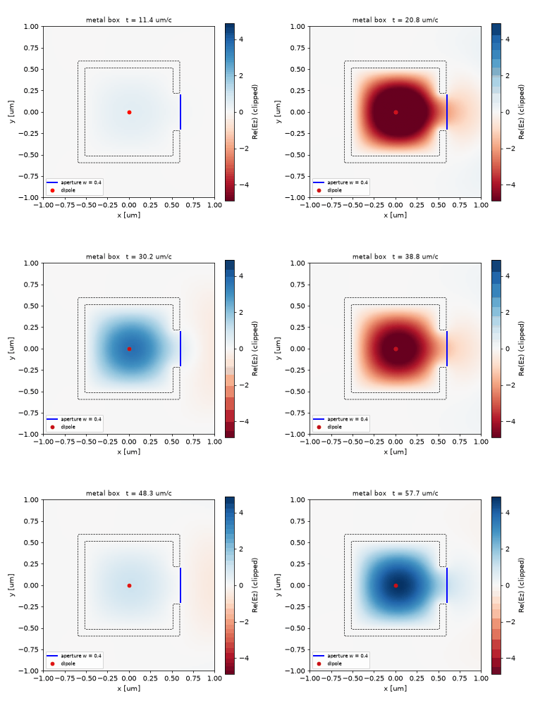
다음으로 파트 B에서는 1 × 1 µm의 2D PEC 상자에 폭 w의 구멍을 냅니다. 구멍이 좁을수록 누설이 줄어 Q가 커지고, 공진 근처 LDOS를 재는 데 필요한 시간도 길어집니다. 이 예제는 2Q/f를 실행 시간의 기준으로 쓰며, 최대 6000에서 자릅니다.
4. 직접 실행하기: 높은 Q를 더 오래 관찰하기
Meep 1.33.0 환경에서 저장소의 code/ 폴더에 있는 원본과 공통 helper를 사용합니다. 먼저 원본 결과를 보관하세요. 기존 단일 코어 실행은 약 6.6분입니다.
OMP_NUM_THREADS=1 python cavity_ldos.py
T_MAX만 6000.0에서 12000.0으로 바꿔 같은 명령으로 실행합니다. 이것은 파트 B의 실행 시간 상한 한 가지만 바꾸는 실험입니다. 다른 파라미터와 source는 그대로 둡니다.
w = 0.2의 로그에서 T_run, dft_ldos, 스펙트럼 폭으로 구한 Q를 원본과 비교하세요. 더 긴 계산에서 공진 스펙트럼이 어떻게 변하는지 확인합니다. 원본이 요구한 시간은 23915이므로 12000 역시 그 기준보다 짧습니다. 새 수치를 수렴한 값으로 단정하지 말고, 원본의 3499.1119와 구별해 기록하세요.
5. 결과 해석하기: 큰 Q와 믿을 수 있는 LDOS는 다르다
| 평면 cavity의 비교 | 실제 기록 |
|---|---|
| cutoff를 제외한 해석식 대비 오차 | 중앙값 0.94%, 최대 3.6% |
| t = 1.0: CYL / 3D / 해석식 | 0.912 / 0.933 / 0.9375 |
| t = 2.0: CYL / 3D / 해석식 | 0.988 / 0.979 / 0.9844 |
| t = 1.5 cutoff의 CYL 값 | 0.507, 아래쪽 해석식 극한 약 0.519에 가까움 |
3D 확인은 t = 1, 2 두 점뿐입니다. 이 일치가 cutoff 근처를 포함한 모든 두께와 해상도의 검증은 아닙니다. t = 2.5의 CYL 값 1.172는 아래쪽 0.728과 위쪽 1.320 사이에 있어, 한쪽 계단에 정확히 일치한다고 말할 수 없습니다.
| 2D 상자의 구멍 w | Harminv Q | 시간 기준 2Q/f | 실행 시간 | LDOS / (Q/V 기반 추정) |
|---|---|---|---|---|
| 0.2 µm | 8060 | 23915 | 6000, 상한 도달 | 0.72 |
| 0.3 µm | 1271 | 3802 | 3802 | 0.89 |
| 0.4 µm | 189 | 574 | 574 | 0.85 |
| 0.5 µm | 74 | 230 | 230 | 0.81 |
표의 근사값은 2Q/(πωV)이며, V = a²/4는 닫힌 상자의 해석값입니다. 구멍이 있는 상자에는 근사이므로 충분히 실행해도 비가 정확히 1일 필요는 없습니다. w = 0.2에서는 시간까지 부족해 스펙트럼 Q가 5597로 Harminv의 8060보다 작았습니다. 따라서 raw LDOS 3499를 수렴한 값으로 보고하지 않습니다.
6. 이해 확인하기
- cavity의 LDOS 하나만 알고 있을 때 “방출이 몇 배 변했다”고 말할 수 없는 이유는 무엇인가요?
- w = 0.2에서 Q가 8060으로 측정되었는데도 LDOS를 수렴한 값으로 보고할 수 없는 이유는 무엇인가요?
두 질문의 답 확인하기
- 같은 매질·source·좌표계의 bulk 기준값이 필요합니다. 두 LDOS의 비율이 Purcell 인자이고, raw LDOS 하나에는 정규화 조건이 섞여 있습니다.
- LDOS 실행은 6000에서 잘렸고 시간 기준 2Q/f는 23915입니다. 공진의 긴 시간 응답을 충분히 포함하지 못했으며 스펙트럼 Q도 다릅니다. 큰 Q 자체가 LDOS 수렴을 보증하지 않습니다.
7. 참고 자료와 전체 코드
원본의 해석식, 좌표계별 설정, 자세한 측정 표와 실행 기록은 아래에서 확인할 수 있습니다.
English summary
TL;DR (English)
- What: post 10 put one mirror next to a dipole and the pattern changed. Here the dipole sits between two mirrors and the question is the emitted power itself. Meep measures it as the local density of states (LDOS) at the source point with
dft_ldos. Part A: an in-plane dipole in a dielectric slab (n = 2.4) between two lossless metallic mirrors, the Purcell factor F = LDOS(cavity)/LDOS(bulk) versus the normalized thickness t = nL/λ, swept in cylindrical coordinates and checked in 3D. Part B: a dipole in a 2D metal box with one aperture, where the LDOS at resonance is compared with the single-mode estimate 2Q/(πωV). - Result: away from the three modal cutoffs the cylindrical sweep matches the analytic curve of Abram et al. with a median error of 0.94% (max 3.6%); at the cutoffs t = 0.5, 1.5, 2.5 the LDOS is discontinuous and FDTD lands on one side of the step. Two full-3D points agree with the cylindrical run to 2.3% / 0.9% (t = 1.0 / 2.0). In the metal box the Harminv Q rises from 74 (w = 0.5) to 8060 (w = 0.2); the directly measured LDOS is 0.81–0.89 of 2Q/(πωV) where the run was long enough, and only 0.72 of it for w = 0.2, whose required run time 2Q/f = 23915 was capped at 6000.
- Takeaway: a mirror changes not only where light goes but how much is emitted. The Purcell factor is always a ratio of two LDOS runs with the same source. A new cavity mode opens at every half wavelength and the LDOS jumps there. A high-Q LDOS costs a run time of order 2Q/f, and an under-converged LDOS is not a small error but a different number.
- Code: full script at the bottom, ~6.6 min on one core.
배경·물리식·파라미터 자세히 보기
원본 §0 · 이 글에서 배우는 것
- LDOS가 무엇인가: 단위 쌍극자가 그 자리에서 내는 power.
dft_ldos는 공간 monitor 없이 source 점에서 이것을 잰다 - Purcell 인자는 LDOS 하나가 아니라 같은 source로 돌린 두 run(cavity, bulk)의 비율이라는 것
- 두 거울 사이에서 반파장마다 모드가 하나씩 열리고 LDOS가 계단처럼 뛰는 이유. cutoff에서는 비교 자체가 성립하지 않는다
- in-plane 쌍극자를 cylindrical 좌표의
Er,m = -1로 표현하는 법(13편의 예고)과 3D와의 교차검증 - z 방향에 PML을 두지 않는 것이 실수가 아니라 거울이라는 물리 조건이라는 것
- 공진 LDOS ≈ 2Q/(πωV). Harminv의 Q로 필요한 run 시간 2Q/f를 정하고, 짧게 돌리면 어떻게 틀리는지
전제 지식: 10편의 image dipole과 PEC, 01편의 점원. 공식 예제: Local density of states 튜토리얼의 planar cavity with lossless metallic walls와 metal cavity with an aperture, 스크립트 planar_cavity_ldos.py · metal-cavity-ldos.py. 이전 글: 10 · 점광원의 3D 방사 패턴 · 다음 글: 12 · 빛을 가두는 고리
원본 §1 · 무엇을 알고 싶은가
10편의 끝 질문이었다. 거울 하나는 방사 패턴을 다섯 lobe로 바꿨다. 거울 둘 사이에 점광원을 두면 패턴만이 아니라 내는 빛의 양 자체가 바뀌는가. 같은 쌍극자, 같은 진폭인데 주변 구조에 따라 power가 달라진다는 것은 고전 전자기학 안에서 설명된다. 쌍극자가 내는 power는 자기 자신이 만든 field가 자기 전류에 하는 일이고, 거울이 그 field를 되돌려 보내면 일의 양이 바뀐다. 이 양을 재는 물리량이 LDOS이고, bulk 대비 비율이 Purcell 인자다. 두 번째 질문은 가둬 둔 빛에 관한 것이다. 금속 상자에 작은 구멍 하나를 내면 빛이 오래 머물고(Q), 그만큼 LDOS가 커진다는 Q/V 관계가 실제 측정과 맞는가.
어디에 쓰이는가
빛을 가두는 이유는 세 가지다. 첫째, 방출 속도가 바뀐다. 발광 분자가 비발광 경로보다 빨리 빛을 내면 효율이 오른다(Purcell). 둘째, 상호작용 시간이 늘어난다. 같은 재료라도 빛이 Q번 왕복하면 센서·변조기·비선형 효과가 Q배 커진다. 셋째, 주파수를 고른다. 공진 주파수의 빛만 통과시키는 것이 필터와 레이저의 원리다. 이 글의 LDOS와 Q는 세 가지 모두의 기초 수치다.
| 응용 | 이 글의 어떤 것을 쓰는가 | 그 다음에 필요한 것 |
|---|---|---|
| OLED·LED 내부 효율 | Purcell 인자. 전극(거울)과 발광층 두께가 방출 속도를 정한다 | 14편 광추출 효율 |
| 단일광자원(양자점–cavity), 레이저 threshold | LDOS, Q/V, 공진 모드의 β 인자 | 12편 고리, 13편 cylindrical |
| 센서·변조기·비선형 소자 | Q로 상호작용 시간을 늘린다 | 12편 ring, 22편 비선형 |
| 필터·파장 분할 다중화(WDM) | 공진 주파수 선택, 선폭 f/Q | 12편 ring resonator |
| 열방사·복사 냉각 | LDOS 그 자체(열 LDOS) | — |
원본 §2 · 물리 한 페이지
주파수 ω에서 위치 $\mathbf x_0$의 쌍극자 $\hat p$가 내는 power는 그 자리의 전기장이 전류에 하는 일 $-\tfrac12\mathrm{Re}[\hat E\cdot\hat J^*]$에 비례한다. Meep의 dft_ldos는 이것을 단위 쌍극자로 정규화해 돌려준다.
분모가 필요한 이유는 분자에 source 진폭, 좌표계, 격자의 정규화가 모두 들어 있기 때문이다. 같은 source 표현으로 bulk를 한 번 더 돌려 나누면 그것들이 상쇄된다. 두 거울 사이의 in-plane 쌍극자에 대해 Abram 등(1998)은 두께 $t=nL/\lambda$의 함수로 닫힌 식을 줬다.
\[F_P(t)=\frac{3N}{4t}+\frac{4N^3-N}{16t^3},\qquad N=\mathrm{fix}\!\left(t+\tfrac12\right)\]$N$은 거울 사이에 들어가는 모드의 수다. $t$가 반정수를 지날 때마다 모드가 하나 열리고 $F_P$가 뛴다. $t=0.5$에서 3, $t=1.0$에서 0.94, $t=2.0$에서 0.98이다. 뛰는 지점(cutoff)에서는 LDOS가 연속 함수가 아니므로 유한 시간·유한 격자의 FDTD 값은 계단의 어느 쪽에 걸리느냐로 정해진다.
금속 상자의 공진 모드 하나가 LDOS를 지배하면 single-mode 근사가 성립한다.
\[\mathrm{LDOS}(\omega_n)\approx\frac{2}{\pi\,\omega_n}\,\frac{Q_n}{V_n},\qquad V^{(1)}=\frac{a^2}{4},\quad \omega^{(1)}=\frac{\sqrt2\,\pi c}{a}\]빛이 오래 머물수록($Q$), 좁은 곳에 몰릴수록($V$) 쌍극자가 더 많이 낸다. dft_ldos로 이것을 직접 재려면 DFT가 수렴할 만큼, 즉 field가 다 빠져나갈 만큼 돌려야 하고 그 시간은 $2Q/f$ 정도다.
| 기호 | 뜻 | 코드 변수 |
|---|---|---|
| $t=nL/\lambda$ | 매질 안 파장 단위의 거울 간격 | T_NORM |
| $L$ | 실제 거울 간격 $t\lambda/n$ | cavity_um |
| $N$ | 열린 모드 수 $\mathrm{fix}(t+\tfrac12)$ | np.fix(t + 0.5) |
| $F_P$ | Purcell 인자 | purcell_cyl, purcell_3d |
| $Q$, $f$ | 공진의 Q와 주파수 (Harminv) | Q, f |
| $V$ | 모드 부피 $a^2/4$ (해석값) | V_MODE |
| $2Q/f$ | dft_ldos에 필요한 run 시간 |
T_req |
가정과 유효 범위: 파트 A는 손실 없는 유전체(n = 2.4)와 완전도체 거울, 단일 주파수, 수평 편광 쌍극자. 파트 B는 2D Ez, 완전도체 상자. 모드 부피 $a^2/4$는 닫힌 상자의 해석값이라 구멍이 있는 상자에는 근사다. 손실 매질의 점광원 LDOS는 해상도에 따라 발산하므로 이 글의 방법을 그대로 옮기면 안 된다.
결과 보기 전에 맞춰보기
| 물리량 | 내 예측 | 근거 |
|---|---|---|
| $F_P(t=1.0)$ | 0.94 | Eq. 7, $N=1$ |
| cutoff 제외 median 오차 (CYL) | 2% 안 | 노트 0.95% |
| cutoff 세 점 | Eq. 7과 다르다, 어느 쪽 계단인지는 모른다 | 불연속점 |
| 3D(res 48) vs CYL, $t=1,2$ | 3% 안 | 노트의 CYL–3D median 1.3% |
| $Q$의 w 의존 | w 0.5 → 0.2에서 수십 배 | 구멍이 좁을수록 누설이 준다 |
| $Q$(w = 0.2) | 8000 근처 | 노트 8060 |
| converged run의 LDOS vs $2Q/(\pi\omega V)$ | 20% 안 | 노트 median 15%. $V$가 근사값 |
| w = 0.2 (cap 6000 < 2Q/f) | $2Q/(\pi\omega V)$의 절반 아래 | 노트: 2000 run에서 62% |
| 스펙트럼 FWHM의 $Q$ vs Harminv $Q$ | 10% 안 | 같은 공진 |
판정 기준: cutoff 밖 median > 5%면 bulk 정규화나 경계(z PML 유무)를 의심한다. converged run에서 LDOS/(Q/V 추정)이 2배 넘게 다르면 Harminv가 다른 모드를 잡은 것이다.
원본 §3 · 시뮬레이션 설계도
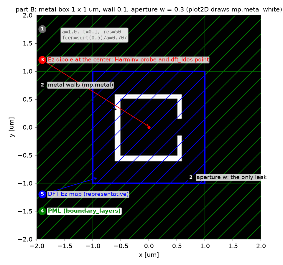
dft_ldos의 점이다. 사방 PML 1 µm. plot2D는 mp.metal(ε = −∞)을 흰색으로, 공기를 검게 그리므로 흰 테두리가 금속이다. 파란 사각형은 대표 Ez DFT 영역.| 파라미터 | 값 | 왜 이 값인가 | 바꾸면 |
|---|---|---|---|
| A 파장, n, 해상도 | 1 µm, 2.4, res 71 | 공식 값. 매질 안 파장 0.417 µm에 30칸 | res가 낮으면 셀 두께가 격자에 반올림되어 계단이 생긴다 |
| A 두께 sweep | $t$ = 0.5~2.5, 0.1 간격 21점 | 공식 41점의 절반. cutoff 세 점 포함 | 간격을 줄이면 cutoff 근처 계단이 더 보인다 |
| A 3D 확인 | $t$ = 1.0, 2.0, res 48 | 전체 sweep을 3D로 하면 수십 분 | 두 점만으로 좌표계 교차검증 |
| A bulk 셀 | CYL 6 µm, 3D 3 µm (+PML 0.5) | 균일 매질이라 크기에 둔감 | 너무 작으면 PML 반사가 LDOS에 섞인다 |
| A 종료 | source 점의 field 감쇠 1e-6 | 공식 값 | cavity run은 z 손실이 없어 bulk보다 오래 걸린다 |
| B 상자, 구멍 | a = 1, 벽 0.1, w = 0.2/0.3/0.4/0.5 | 공식 0.2~0.4에 0.5 추가 | w가 작을수록 Q와 필요한 시간이 커진다 |
| B Harminv | fcen = √0.5/a = 0.707, df 0.2, 500 time unit | 닫힌 상자의 기본 모드 주파수 | 대역을 넓히면 고차 모드가 섞인다 |
B dft_ldos 시간 |
min(2Q/f, 6000) | 공식은 cap 없음. w = 0.2는 일부러 미수렴 | cap을 없애면 w = 0.2가 수십 분 |
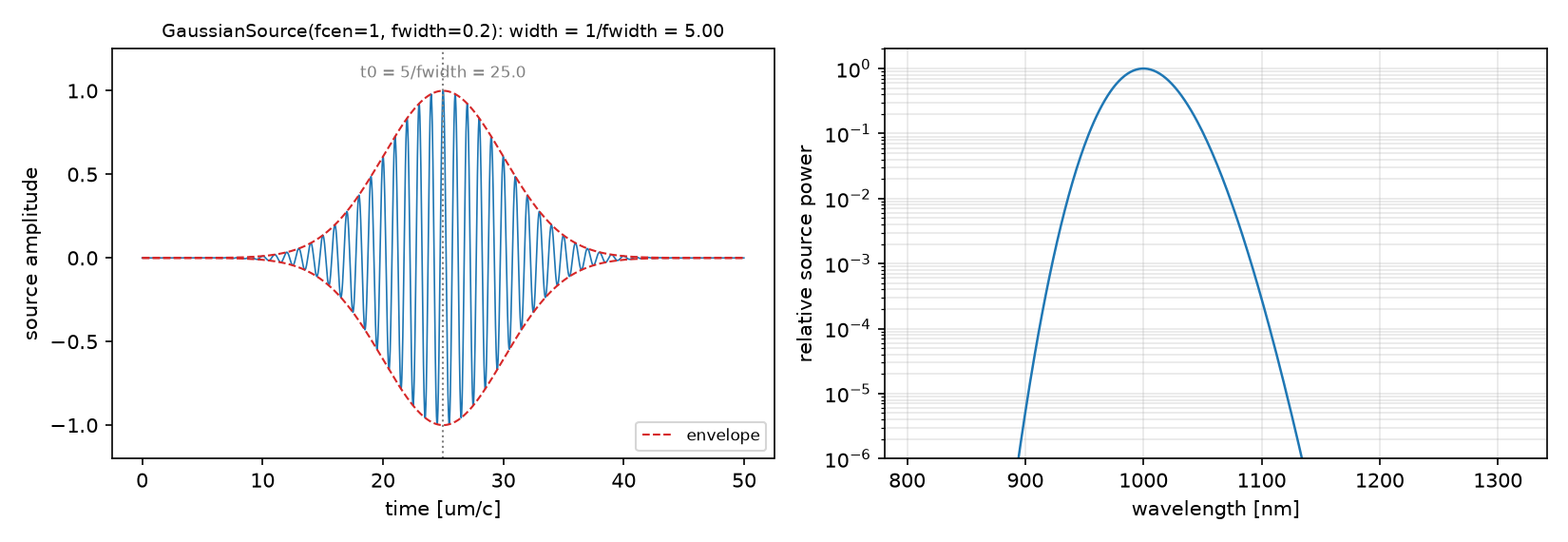
강의 노트북과의 차이: 강의 범위 밖이다. 10_sources의 두 노트는 각각 41점 sweep(CYL + 3D 전체, res 71)과 구멍 세 개(2000 cap)를 돌렸다. 이 글은 sweep을 21점으로 줄이고 3D를 두 점으로 제한한 대신, 구멍에 w = 0.5를 더하고 dft_ldos 스펙트럼의 폭으로 Q를 한 번 더 재서 Harminv와 맞춘다.
원본 코드 단계별 설명
원본 §4 · 코드 따라가기
읽는 순서: 단위·파라미터 → 재료·구조 → source → Simulation·경계 → monitor → 실행·종료 → 후처리. 이번 글의 ⑤는 공간 monitor가 아니라 source 점의
dft_ldos와Harminv다.
① 단위와 파라미터 — 어떤 숫자를 고정하는가
WL, N_CAV, RES_CYL, RES_3D = 1.0, 2.4, 71, 48
T_NORM = np.round(np.arange(0.5, 2.51, 0.1), 2)       # t = n L / wl; cutoffs at 0.5, 1.5, 2.5
L = t * WL / N_CAV                                     # the physical mirror spacing that goes into the cell

A_BOX, T_WALL, WS = 1.0, 0.1, (0.2, 0.3, 0.4, 0.5)     # metal box, wall, aperture widths
FCEN_M = math.sqrt(0.5) / A_BOX                        # fundamental mode of the closed box
T_MAX = 6000.0                                         # cap on the dft_ldos run
- 무엇: 파트 A의 두께 sweep과 해상도, 파트 B의 상자와 구멍 폭.
- 왜: 그림의 가로축은 물리 두께가 아니라 $t=nL/\lambda$다. 셀에는 $L=t\lambda/n$을 넣어야 한다. 상자의 기본 모드는 $\omega=\sqrt2\pi c/a$, 즉 $f=\sqrt{0.5}/a$이고 Harminv의 중심이 된다.
- 틀리면: $t$를 µm로 그대로 넣으면 거울 간격이 2.4배 넓어지고 Eq. 7과 비교할 수 없다.
② 재료와 구조 — 거울은 PML을 두지 않은 벽
# part A, cavity: PML only in r (cyl) or x, y (3D). The z walls of the cell are Meep's default PEC = the mirrors.
pml = [mp.PML(thickness=DPML, direction=mp.R)]
# part A, bulk: PML on every side, same source, same medium
pml = [mp.PML(thickness=DPML)]
# part B: a metal shell, an air box, and an air block that cuts the aperture into the right wall
geometry = [mp.Block(mp.Vector3(A_BOX + 2 * T_WALL, A_BOX + 2 * T_WALL, mp.inf), material=mp.metal),
            mp.Block(mp.Vector3(A_BOX, A_BOX, mp.inf), material=mp.air),
            mp.Block(center=mp.Vector3(A_BOX / 2), size=mp.Vector3(2 * T_WALL, w, mp.inf), material=mp.air)]
- 무엇: 파트 A의 거울은 geometry가 아니다. z 방향에 PML이 없으면 셀 벽이 완전도체이고 그것이 거울이다. bulk run은 모든 방향을 PML로 열어 거울을 없앤다. 파트 B는 금속 블록 → 공기 블록 → 구멍 블록 순으로 덮어쓴다.
- 왜: Purcell 인자는 “거울이 있을 때 / 없을 때”의 비율이다. 두 run의 차이가 경계 조건 하나뿐이어야 한다.
- 틀리면: cavity run에 z PML을 두면 run은 더 빨리 끝나지만 거울이 없어진다. 10편의 반대 경우다. 그때는
k_point때문에 벽이 거울이 아니었고, 여기서는k_point가 없어 벽이 거울이다.
③ Source — in-plane 쌍극자의 두 표현
# cyl: an x-dipole is the m = -1 family of Er; the axis r = 0 is singular, so offset by 1.5 pixels
src_pt = mp.Vector3(1.5 / RES_CYL, 0, 0)
sources = [mp.Source(mp.GaussianSource(FCEN, fwidth=FWIDTH), component=mp.Er, center=src_pt)]
# 3D: the same dipole as Ex at the origin
sources = [mp.Source(mp.GaussianSource(FCEN, fwidth=FWIDTH), component=mp.Ex, center=mp.Vector3())]
- 무엇: 같은 물리 쌍극자를 cylindrical에서는
Er,m = -1로, 3D에서는Ex로 둔다. - 왜: x 방향 쌍극자의 방위각 의존성은 $e^{\pm i\phi}$, 즉 $m=\pm1$이다. 축 위에서는 r 방향 단위벡터가 정의되지 않으므로 1.5 픽셀 비킨다. 이 offset은 구조 변경이 아니라 좌표 특이점 회피다.
- 틀리면: offset을 µm 상수로 고정하면 해상도를 바꿀 때 픽셀 단위 표현이 달라진다. 13편에서 cylindrical 좌표를 본격적으로 다룬다.
④ Simulation과 경계 — CYL의 m과 3D의 symmetry 위상
sim = mp.Simulation(resolution=RES_CYL, cell_size=mp.Vector3(cell_r, 0, cell_z), boundary_layers=pml,
                    dimensions=mp.CYLINDRICAL, m=-1, default_material=mp.Medium(index=N_CAV), sources=sources)

sim = mp.Simulation(..., symmetries=[mp.Mirror(mp.X, phase=-1), mp.Mirror(mp.Y), mp.Mirror(mp.Z)])   # 3D: Ex is odd under x
- 무엇: cylindrical은
dimensions=mp.CYLINDRICAL과m. 3D는 세 거울 대칭으로 계산을 1/8로. - 왜:
Ex는 x 반전에서 부호가 바뀌고 y, z 반전에서는 그대로다. 위상은 geometry가 아니라 source 벡터의 parity다. - 틀리면: 위상을 전부 +1로 두면 더 빠른 같은 계산이 아니라 다른 parity의 source를 계산한다. 10편의 image dipole에서 Ez가 odd였던 것과 같은 규칙이다.
⑤ Monitor — 공간 monitor 없이 source 점에서
sim.run(mp.dft_ldos(FCEN, 0, 1), until_after_sources=...)          # LDOS at one frequency, at the source point
ldos = sim.ldos_data[0]

h = mp.Harminv(mp.Ez, mp.Vector3(), FCEN_M, DF_M)                   # part B: f and Q of the ringing field
sim.run(mp.after_sources(h), until_after_sources=500)
f, Q = h.modes[0].freq, h.modes[0].Q
sim.run(mp.dft_ldos(f, 8 * f / Q, 101), until_after_sources=min(2 * Q / f, T_MAX))   # spectrum +-4 linewidths around f
- 무엇:
dft_ldos는 step function이다. source 점의 field와 전류의 DFT를 축적해 LDOS를 만든다. Harminv는 source가 꺼진 뒤의 감쇠에서 공진 주파수와 Q를 꺼낸다. - 왜: LDOS는 flux가 아니라 source 자리의 일이다. 그래서 flux box가 필요 없고 source 점 하나면 된다. 파트 B에서는 Harminv의 f를
dft_ldos의 주파수로 넘기고, 스펙트럼의 폭으로 Q를 한 번 더 확인한다. - 틀리면:
dft_ldos의 주파수를 Harminv의 f가 아니라 처음의 fcen으로 두면 공진에서 조금 비껴 LDOS가 작게 나온다. Q가 수천이면 폭이 1e-4라 조금이 크다.
⑥ 실행 — 감쇠 조건과 2Q/f
until_after_sources=mp.stop_when_fields_decayed(20, mp.Er, src_pt, 1e-6)    # part A
until_after_sources=min(2 * Q / f, T_MAX)                                     # part B
- 무엇: 파트 A는 source 점의 field가 1e-6으로 줄 때까지. 파트 B는 Q로 정한 시간만큼.
- 왜: Fourier 불확정성 때문에 선폭 $f/Q$를 분해하려면 감쇠 시간 한 주기, $2Q/f$가 필요하다. w = 0.2의 Q는 8000 근처라 $2Q/f\approx 23000$이고, 이 글은 6000에서 자른다. 그 결과가 어떻게 틀리는지를 보여 주기 위해서다.
- 틀리면: cavity run을 bulk run처럼 짧게 끝내면 거울 사이에 남은 field가 LDOS에 다 더해지지 못한다. 파트 A의 cavity run이 bulk보다 오래 걸리는 것은 정상이다.
⑦ 후처리 — 비율, Eq. 7, Q/V
purcell = ldos_cavity / ldos_bulk                                      # same source, same medium, same coordinates
N = np.fix(t + 0.5); theory = 3 * N / (4 * t) + (4 * N**3 - N) / (16 * t**3)
cutoff = np.isclose(np.mod(t, 1.0), 0.5)                               # exclude from the error statistics, keep the raw values

ldos_qv = Q / V_MODE / (2 * math.pi * f * math.pi * 0.5)               # 2Q / (pi w V), V = a^2 / 4
- 무엇: Purcell은 비율. Eq. 7과의 오차는 cutoff를 빼고 median과 max를 함께 적는다. 파트 B는 Q/V 추정과 직접 측정을 나란히 둔다.
- 왜: median만 적으면 $t=1.45$ 같은 국소 실패가 가려진다. cutoff 값은 버리지 않고 표로 남긴다.
- 틀리면: cutoff의 FDTD 값을 “틀렸다”고 분류하거나 유리한 쪽 계단으로 바꾸면 안 된다. 그 점의 해석값 자체가 두 개다.
함정: Meep은 셀 크기를 픽셀 정수로 반올림한다. $L\times$res가 정수가 아니면 이웃한 두께가 같은 z 격자 수를 쓰게 되어 sweep 곡선에 작은 계단이 생긴다. cutoff 근처에서는 이 반올림이 열린 모드의 표현을 바꿀 수 있다. 로그의 “cell size will be rounded”는 무시할 문자열이 아니다.
원본 결과·검증 표·오류 진단·추가 탐구
원본 §5 · 결과
| $t$ | Eq. 7 | CYL | 3D (res 48) | 비고 |
|---|---|---|---|---|
| 0.5 | 3.000 | 3.018 | — | cutoff |
| 1.0 | 0.9375 | 0.912 | 0.933 | |
| 1.5 | 1.556 (위 계단) / 0.519 (아래) | 0.507 | — | cutoff. FDTD는 아래 계단 |
| 2.0 | 0.9844 | 0.988 | 0.979 | |
| 2.5 | 1.320 (위) / 0.728 (아래) | 1.172 | — | cutoff |
| cutoff 제외 18점 | — | median 0.94%, max 3.6% (t = 0.70) | — |
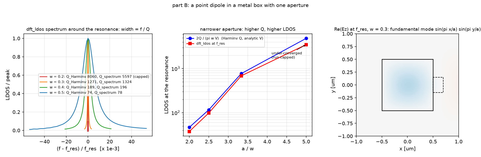
dft_ldos 스펙트럼. 폭이 $f/Q$다. 가운데: Q/V 추정(파랑)과 직접 측정(빨강)을 a/w에 대해 semilog로. w = 0.2는 run을 잘라 미수렴. 오른쪽: w = 0.3의 공진 Ez. 닫힌 상자의 기본 모드 $\sin(\pi x/a)\sin(\pi y/a)$에 구멍 쪽 누설이 더해진 모양.| w | f (Harminv) | Q (Harminv) | Q (스펙트럼 폭) | 2Q/f | 실행 | $2Q/(\pi\omega V)$ | dft_ldos |
비 |
|---|---|---|---|---|---|---|---|---|
| 0.2 | 0.6740 | 8060 | 5597 (잘린 run) | 23915 | 6000 (cap) | 4846 | 3499 | 0.72 |
| 0.3 | 0.6688 | 1271 | 1324 | 3802 | 3802 | 770 | 686 | 0.89 |
| 0.4 | 0.6569 | 189 | 196 | 574 | 574 | 116 | 98 | 0.85 |
| 0.5 | 0.6465 | 74 | 78 | 230 | 230 | 46.7 | 37.6 | 0.81 |
예측과 비교
| 물리량 | 내 예측 (§2) | 시뮬레이션 | 판정 |
|---|---|---|---|
| $F_P(t=1.0)$ | 0.94 | 0.912 | ✅ (2.7% 차) |
| cutoff 제외 median 오차 | 2% 안 | 0.94% | ✅ |
| cutoff 세 점 | Eq. 7과 다름 | 0.5: 3.018, 1.5: 0.507, 2.5: 1.172 | cutoff: 1.5는 아래쪽에 가깝고, 2.5는 두 극한 사이 |
| 3D vs CYL | 3% 안 | 2.3% / 0.9% (t = 1.0 / 2.0) | ✅ |
| $Q$의 w 의존 | 수십 배 | 74 → 8060 | ✅ (109배) |
| $Q$(w = 0.2) | 8000 근처 | 8060 | ✅ |
| converged LDOS vs Q/V | 20% 안 | 0.81~0.89 | ✅ |
| w = 0.2 미수렴 | 절반 아래 | 0.72 (28% 부족) | ❌ (절반보다 위) |
| 스펙트럼 Q vs Harminv Q | 10% 안 | 1324/1271, 196/189, 78/74 (4~5%) | ✅ |
아홉 예측 중 여덟이 맞았다. 틀린 것은 w = 0.2의 미수렴 정도다. 노트는 필요 시간의 8%(2000)만 돌려 62%가 모자랐고, 이 글은 25%(6000)를 돌려 28%가 모자랐다. run을 자르면 공진 봉우리의 꼬리가 DFT에 다 들어오지 못해 LDOS가 작아지고 스펙트럼은 넓어진다. 스펙트럼 폭으로 잰 Q가 5597로 Harminv의 8060보다 작은 것이 그 지문이다. 나머지 세 구멍에서는 스펙트럼 Q와 Harminv Q가 5% 안에서 같고, 직접 잰 LDOS는 Q/V 추정의 81~89%다. 남은 10~20%는 모드 부피 $a^2/4$가 닫힌 상자의 값이라 구멍이 넓을수록 실제 모드가 더 퍼지기 때문이고, 실제로 w가 넓어질수록 비가 0.89에서 0.81로 내려간다. 파트 A에서 $t=1.0$의 CYL 값 0.912는 Eq. 7의 0.9375보다 2.7% 낮지만 3D 값 0.933이 그 사이에 있어 좌표계 표현의 차이로 본다. cutoff에서는 예측대로 FDTD가 계단의 한쪽에 걸렸다. $t=0.5$는 위 계단(3.018 vs 3.0), $t=1.5$는 아래쪽 극한에 가깝고(0.507 vs 0.519), $t=2.5$의 1.172는 아래쪽 0.728과 위쪽 1.320 사이이다.
수렴성
| 변수 | 값 | 결과 | 비고 |
|---|---|---|---|
| A sweep 간격 | 0.1 (21점, 이 글) vs 0.05 (41점, 노트) | median 0.94% vs 0.95% | 간격은 오차를 바꾸지 않는다. 각 점이 독립 run |
| A 3D 해상도 | 48 (이 글) vs 71 (노트) | $t=1,2$에서 CYL과 2.3% / 0.9% (t = 1.0 / 2.0) vs 노트 median 1.3% | 노트의 3D max 11.4%($t=1.45$)는 이 글에서 재지 않았다 |
| B run 시간 | 2Q/f (w ≥ 0.3) vs cap 6000 (w = 0.2) | 비 0.81~0.89 vs 0.72 | 미수렴은 작은 오차가 아니라 다른 숫자 |
주장할 수 있는 것 / 없는 것
- 할 수 있는 것: n = 2.4, 완전도체 거울, res 71에서 cylindrical
dft_ldos의 Purcell 인자는 cutoff 밖에서 Eq. 7 대비 상대오차 중앙값 0.94%, 최대 3.6%이며, 3D 두 점과 2.3% / 0.9% (t = 1.0 / 2.0) 안에서 같다. 금속 상자에서 Harminv의 Q로 정한 시간만큼 돌리면 직접 잰 LDOS가 $2Q/(\pi\omega V)$와 0.81~0.89 안에서 같다. - 할 수 없는 것: cutoff 세 점의 값. 해석식 자체가 불연속이다. 노트가 본 3D의 국소 11% 오차($t=1.45$)는 이 글의 두 점에 없다. 손실 있는 거울이나 매질. 모드 부피 $a^2/4$는 닫힌 상자의 값이라 구멍이 넓어질수록 근사가 나빠진다. w = 0.2의 LDOS는 이 글의 run 시간으로는 모른다.
원본 §6 · 흔한 실수
| 증상 | 원인 | 고치는 법 |
|---|---|---|
| Purcell이 전부 1 근처 | cavity run에 z PML을 둠(거울 없음) | cavity는 횡방향만 PML, bulk는 전방향 |
| Purcell이 수십 배 | bulk 정규화를 빼먹고 raw LDOS를 봄 | 같은 source로 bulk를 돌려 나눈다 |
| CYL run이 축에서 발산 | Er를 r = 0에 둠 |
1.5 픽셀 offset |
| 3D 결과가 CYL과 2배 다름 | symmetry 위상 전부 +1 | Ex는 Mirror(X, phase=-1) |
| sweep 곡선의 작은 계단 | 셀 두께가 픽셀로 반올림 | $L\times$res가 정수가 되게 고르거나 해상도를 올린다 |
| cutoff에서 50% 오차 | 불연속점을 일반 점처럼 통계에 넣음 | raw 값은 남기고 median에서 뺀다 |
| 직접 LDOS가 Q/V의 절반 | dft_ldos run이 2Q/f보다 짧음 |
Q를 먼저 재고 시간을 정한다 |
| r–z field 그림이 뒤집힘, 한 줄만 진함 | cylindrical의 get_array·get_dft_array는 (z, r) 순서 |
2D처럼 전치하지 않는다. 진한 한 줄은 r = 0의 source 열 |
| field 그림이 거의 비어 보임 | source 픽셀이 색 범위의 최대값을 차지 | 99 percentile로 색 범위를 자른다 |
| LDOS가 공진값보다 작음 | dft_ldos 주파수를 Harminv의 f가 아니라 fcen으로 |
Harminv f를 넘긴다 |
원본 §7 · 직접 해보기
| 바꿀 것 | 예상 변화 | 확인할 수치 |
|---|---|---|
파트 A의 쌍극자를 z 방향(Ez, m = 0)으로 |
수직 쌍극자는 거울 사이에서 다른 곡선 | $t<0.5$에서 0이 아닌지 |
| sweep 간격 0.1 → 0.02, $t$ = 1.4~1.6 | cutoff 1.5 근처의 계단 모양 | 어느 $t$에서 뛰는지 |
| 파트 A 해상도 50 / 71 / 100 | cutoff 밖 median의 사다리 | 0.94%가 어디서 정체하는지 |
| 파트 B의 cap을 없애고 w = 0.2 | 비가 1 근처로 | 비, 걸린 시간 |
| 파트 B에 w = 0.1 | Q 수만, 2Q/f 수십만 | Harminv만으로 Q/V 추정 |
code/cavity_ldos.py 전체 (클릭하여 펼치기)
"""Meep Example 11 - A point dipole between two mirrors: LDOS and the Purcell factor.

Post 10 showed that one mirror rewrites the radiation pattern. Here the dipole sits between two mirrors and the
question is the emitted POWER itself, measured as the local density of states (LDOS) at the dipole position.
  A. Planar cavity (official planar_cavity_ldos.py): lossless metallic walls, dielectric n = 2.4, in-plane dipole.
     The Purcell factor F = LDOS(cavity) / LDOS(bulk) versus the normalized thickness t = n L / wl, swept in
     cylindrical coordinates (Er, m = -1 represents an x-dipole) and checked at two thicknesses in full 3D.
     Compared with the analytic Eq. 7 of Abram et al. (1998): F = 3N/(4t) + (4N^3 - N)/(16 t^3), N = fix(t + 1/2).
  B. Metal box with an aperture (official metal-cavity-ldos.py, 2D): Harminv gives f and Q of the fundamental mode;
     the LDOS at f is measured directly with dft_ldos and compared with the single-mode estimate 2Q/(pi w V).
     The required run time 2Q/f grows with Q; the narrowest aperture is deliberately left under-converged.

Run:  python cavity_ldos.py       (~15 min on one core)
Out:  00_source.png, 01_layout.png, 02_layout_cyl.png, 03_purcell.png, 04_cavity_field.png, 05_metal_ldos.png,
      06_anim_planar.gif, 07_anim_metal.gif, result.json   (-> ../assets/11/)
"""
import json
import math
import os
import sys
import time

import numpy as np
import matplotlib
matplotlib.use("Agg")
import matplotlib.pyplot as plt
import meep as mp

sys.path.insert(0, os.path.dirname(os.path.abspath(__file__)))
from blogfig import Label, _badge, animate_fields, annotated_layout, record_frames, source_figure   # noqa: E402

HERE = os.path.dirname(os.path.abspath(__file__))
OUT = os.path.join(HERE, "..", "assets", "11")
os.makedirs(OUT, exist_ok=True)
t_all = time.time()

# =================================================================== A. planar cavity with lossless metallic walls
# ---------------------------------------------------------------- (1) parameters (official values; 21-point sweep instead of 41)
WL = 1.0
FCEN = 1 / WL
FWIDTH = 0.2 * FCEN
N_CAV = 2.4
RES_CYL = 71
RES_3D = 48                              # 3D cross-check only (official: 71)
DPML = 0.5
BULK_CYL, BULK_3D = 6.0, 3.0
DECAY_TOL, DECAY_PERIOD = 1e-6, 20
T_NORM = np.round(np.arange(0.5, 2.51, 0.1), 2)          # t = n L / wl; cutoffs at 0.5, 1.5, 2.5
T_3D = (1.0, 2.0)                                         # thicknesses checked in full 3D


def purcell_theory(t):
    N = np.fix(t + 0.5)
    return 3 * N / (4 * t) + (4 * N ** 3 - N) / (16 * t ** 3)


def ldos_cyl(cavity_um=None, *, want_field=False):
    """LDOS of an in-plane dipole (Er, m = -1) in cylindrical coordinates; bulk medium if cavity_um is None."""
    if cavity_um is None:
        cell_z, pml = BULK_CYL + 2 * DPML, [mp.PML(thickness=DPML)]
    else:
        cell_z, pml = cavity_um, [mp.PML(thickness=DPML, direction=mp.R)]      # no z PML: the cell walls are the mirrors
    cell_r = BULK_CYL + DPML
    src_pt = mp.Vector3(1.5 / RES_CYL, 0, 0)                                    # Er at r = 0 is singular: offset by 1.5 px
    sim = mp.Simulation(resolution=RES_CYL, cell_size=mp.Vector3(cell_r, 0, cell_z), boundary_layers=pml, dimensions=mp.CYLINDRICAL, m=-1,
                        default_material=mp.Medium(index=N_CAV),
                        sources=[mp.Source(mp.GaussianSource(FCEN, fwidth=FWIDTH), component=mp.Er, center=src_pt)])
    dft = sim.add_dft_fields([mp.Er], FCEN, 0, 1, center=mp.Vector3(0.5 * BULK_CYL, 0, 0), size=mp.Vector3(BULK_CYL, 0, cell_z)) if want_field else None
    sim.run(mp.dft_ldos(FCEN, 0, 1), until_after_sources=mp.stop_when_fields_decayed(DECAY_PERIOD, mp.Er, src_pt, DECAY_TOL))
    ldos = float(sim.ldos_data[0]); t_end = sim.meep_time()
    field = sim.get_dft_array(dft, mp.Er, 0) if want_field else None
    sim.reset_meep()
    return (ldos, t_end, field) if want_field else (ldos, t_end)


def ldos_3d(cavity_um=None):
    """LDOS of an Ex dipole in full 3D (reduced resolution); bulk if cavity_um is None."""
    if cavity_um is None:
        size_z, pml = BULK_3D + 2 * DPML, [mp.PML(thickness=DPML)]
    else:
        size_z, pml = cavity_um, [mp.PML(thickness=DPML, direction=mp.X), mp.PML(thickness=DPML, direction=mp.Y)]
    size_xy = BULK_3D + 2 * DPML
    sim = mp.Simulation(resolution=RES_3D, cell_size=mp.Vector3(size_xy, size_xy, size_z), boundary_layers=pml,
                        default_material=mp.Medium(index=N_CAV),
                        sources=[mp.Source(mp.GaussianSource(FCEN, fwidth=FWIDTH), component=mp.Ex, center=mp.Vector3())],
                        symmetries=[mp.Mirror(mp.X, phase=-1), mp.Mirror(mp.Y), mp.Mirror(mp.Z)])      # Ex is odd under x, even under y, z
    sim.run(mp.dft_ldos(FCEN, 0, 1), until_after_sources=mp.stop_when_fields_decayed(DECAY_PERIOD, mp.Ex, mp.Vector3(), DECAY_TOL))
    ldos = float(sim.ldos_data[0]); t_end = sim.meep_time(); sim.reset_meep()
    return ldos, t_end


source_figure(FCEN, FWIDTH, os.path.join(OUT, "00_source.png"), wl_scale=1000.0, wl_unit="nm", time_unit="um/c")

# layout of the CYL cavity (r-z plane) at t = 1.0, drawn by hand: the cell is 6.5 x 0.42 um, far too thin for plot2D
L_demo = 1.0 * WL / N_CAV
fig, ax = plt.subplots(figsize=(9.5, 3.6))
ax.axvspan(BULK_CYL, BULK_CYL + DPML, color="green", alpha=0.25)
ax.axhline(0.5 * L_demo, color="k", lw=4); ax.axhline(-0.5 * L_demo, color="k", lw=4)
ax.plot(1.5 / RES_CYL, 0, "o", color="red", ms=7); ax.axvline(0, color="gray", ls="-.", lw=1)
for xy, step, color, txt, txy in (((0.25, 0.5 * L_demo - 0.03), 1, "dimgray", f"wl={WL} um, n={N_CAV}, res={RES_CYL}\ncell r {BULK_CYL + DPML} um x z L={L_demo:.3f} um, m=-1", (0.45, 0.5 * L_demo - 0.03)),
                                   ((3.0, 0.5 * L_demo), 2, "black", "top/bottom cell walls: no PML here, so they are PEC = the two mirrors", (3.2, 0.5 * L_demo - 0.035)),
                                   ((1.5 / RES_CYL, -0.035), 3, "red", "Er dipole (m = -1 = an in-plane dipole) at r = 1.5 px, the axis is singular", (0.45, -0.045)),
                                   ((BULK_CYL + 0.5 * DPML, 0.0), 4, "green", "PML (r only)", (BULK_CYL + 0.08, 0.04)),
                                   ((0.4, 0.07), 5, "blue", "LDOS: dft_ldos at the source point (no spatial monitor); bulk run = same cell with PML on z too", (0.6, 0.06)),
                                   ((1.5 / RES_CYL, 0.11), 6, "purple", "decay watch point = source point", (0.45, 0.10))):
    _badge(ax, xy, step, color); ax.text(*txy, txt, fontsize=8, color=color, va="center")
ax.text(0.05, -0.5 * L_demo + 0.01, "r = 0 (axis)", fontsize=7, color="gray", rotation=90, va="bottom")
ax.set_xlim(-0.1, BULK_CYL + DPML); ax.set_ylim(-0.5 * L_demo - 0.02, 0.5 * L_demo + 0.02)
ax.set_xlabel("r [um]"); ax.set_ylabel("z [um]  (stretched)")
ax.set_title("part A: cylindrical r-z cell at t = 1.0. The z axis is stretched 6x; the real cell is a thin disc between two mirrors", fontsize=9)
fig.tight_layout(); fig.savefig(os.path.join(OUT, "02_layout_cyl.png"), dpi=150); plt.close(fig)

t_a = time.time()
bulk_cyl, t_bulk_cyl = ldos_cyl()
purcell_cyl, t_end_cyl, fields = [], [], {}
for t in T_NORM:
    L = t * WL / N_CAV
    if t in (1.0, 2.0):
        ldos, t_end, fld = ldos_cyl(L, want_field=True); fields[t] = (fld, L)
    else:
        ldos, t_end = ldos_cyl(L)
    purcell_cyl.append(ldos / bulk_cyl); t_end_cyl.append(t_end)
purcell_cyl = np.array(purcell_cyl)
theory = purcell_theory(T_NORM)
cutoff = np.isclose(np.mod(T_NORM, 1.0), 0.5)
err_cyl = np.abs(purcell_cyl - theory) / theory
print(f"A (cyl): bulk LDOS {bulk_cyl:.5f} (t_end {t_bulk_cyl:.0f}); {len(T_NORM)} thicknesses in {time.time() - t_a:.0f} s; "
      f"rel error vs Eq. 7 away from cutoffs: median {np.median(err_cyl[~cutoff]):.4f}, max {err_cyl[~cutoff].max():.4f} at t = {T_NORM[~cutoff][np.argmax(err_cyl[~cutoff])]:.2f}; "
      f"at the cutoffs: " + ", ".join(f"t={t:.1f}: Meep {p:.3f} vs Eq.7 {th:.3f}" for t, p, th in zip(T_NORM[cutoff], purcell_cyl[cutoff], theory[cutoff])))

t_a = time.time()
bulk_3d, t_bulk_3d = ldos_3d()
purcell_3d = {}
for t in T_3D:
    ldos, t_end = ldos_3d(t * WL / N_CAV)
    purcell_3d[t] = ldos / bulk_3d
print(f"A (3D, res {RES_3D}): bulk LDOS {bulk_3d:.5f} (t_end {t_bulk_3d:.0f}); " + ", ".join(f"t={t}: 3D {purcell_3d[t]:.4f} vs cyl {purcell_cyl[np.isclose(T_NORM, t)][0]:.4f} vs Eq.7 {purcell_theory(t):.4f}" for t in T_3D)
      + f"; {time.time() - t_a:.0f} s")

fig, ax = plt.subplots(1, 2, figsize=(12, 4.2), gridspec_kw={"width_ratios": [1.5, 1]})
tt = np.linspace(0.5, 2.5, 801)
ax[0].plot(tt, purcell_theory(tt), "-", color="k", lw=1.2, label="Eq. 7 (Abram 1998)")
ax[0].plot(T_NORM, purcell_cyl, "o", color="tab:red", ms=5, label=f"Meep cylindrical (Er, m = -1), res {RES_CYL}")
ax[0].plot(list(T_3D), [purcell_3d[t] for t in T_3D], "s", color="tab:blue", ms=7, label=f"Meep 3D (Ex), res {RES_3D}")
for tc in (0.5, 1.5, 2.5):
    ax[0].axvline(tc, color="gray", ls=":", lw=1)
ax[0].axhline(1, color="gray", ls="--", lw=1); ax[0].text(2.3, 1.03, "bulk", fontsize=8, color="gray")
ax[0].set_xlabel("normalized cavity thickness t = n L / wavelength"); ax[0].set_ylabel("Purcell factor  LDOS(cavity) / LDOS(bulk)")
ax[0].set_title("in-plane dipole between two lossless mirrors (n = 2.4): a new mode opens at every half-integer", fontsize=9)
ax[0].set_ylim(0.4, 3.2); ax[0].grid(alpha=0.3); ax[0].legend(fontsize=8)
ax[1].bar(T_NORM[~cutoff], 100 * err_cyl[~cutoff], width=0.07, color="tab:red", alpha=0.7, label="cylindrical")
ax[1].bar(T_NORM[cutoff], 100 * err_cyl[cutoff], width=0.07, color="lightgray", label="at a cutoff (excluded)")
for t in T_3D:
    ax[1].plot(t, 100 * abs(purcell_3d[t] - purcell_theory(t)) / purcell_theory(t), "s", color="tab:blue", ms=7)
ax[1].set_xlabel("t"); ax[1].set_ylabel("|Meep - Eq. 7| / Eq. 7  [%]"); ax[1].set_title(f"error: median {100 * np.median(err_cyl[~cutoff]):.2f} % away from cutoffs", fontsize=9)
ax[1].grid(axis="y", alpha=0.3); ax[1].legend(fontsize=8)
fig.tight_layout(); fig.savefig(os.path.join(OUT, "03_purcell.png"), dpi=150); plt.close(fig)

fig, ax = plt.subplots(2, 1, figsize=(10, 5.2))
for a, t in zip(ax, (1.0, 2.0)):
    fld, L = fields[t]
    # NOTE: in cylindrical coordinates get_dft_array / get_array return (z, r), not (r, z): no transpose here
    fld = fld[2:-2, :]                                      # drop the two grid rows touching each mirror (boundary pixels of the DFT array)
    nz = fld.shape[0]; dz = L / (nz + 4)
    ext = [0, BULK_CYL, -0.5 * L + 2 * dz, 0.5 * L - 2 * dz]
    lim = float(np.percentile(np.abs(fld), 99.5))           # the source pixel dominates the maximum: clip the colour scale
    a.imshow(np.real(fld), extent=ext, origin="lower", cmap="RdBu", vmin=-lim, vmax=lim, aspect="auto")
    a.axhline(0.5 * L, color="k", lw=2); a.axhline(-0.5 * L, color="k", lw=2); a.plot(1.5 / RES_CYL, 0, "o", color="lime", ms=4)
    a.set_title(f"Re(Er) at t = {t:.1f} (L = {L:.3f} um): F = {purcell_cyl[np.isclose(T_NORM, t)][0]:.3f}   (thick black lines = mirrors)", fontsize=9)
    a.set_ylabel("z [um]")
ax[1].set_xlabel("r [um]")
fig.suptitle("part A: steady-state field between the mirrors, cylindrical r-z plane", fontsize=10)
fig.tight_layout(); fig.savefig(os.path.join(OUT, "04_cavity_field.png"), dpi=150); plt.close(fig)

# GIF: a short pulse between the mirrors at t = 1.0 (r-z plane)
L = 1.0 * WL / N_CAV
fw_anim = 0.5 * FCEN
sim_g = mp.Simulation(resolution=RES_CYL, cell_size=mp.Vector3(BULK_CYL + DPML, 0, L), boundary_layers=[mp.PML(thickness=DPML, direction=mp.R)],
                      dimensions=mp.CYLINDRICAL, m=-1, default_material=mp.Medium(index=N_CAV),
                      sources=[mp.Source(mp.GaussianSource(FCEN, fwidth=fw_anim), component=mp.Er, center=mp.Vector3(1.5 / RES_CYL, 0, 0))])
sim_g.init_sim()
vol_g = mp.Volume(center=mp.Vector3(0.5 * BULK_CYL, 0, 0), size=mp.Vector3(BULK_CYL, 0, L))
t0g = 5 / fw_anim
frames, times = record_frames(sim_g, vol_g, mp.Er, t_start=t0g - 2 / fw_anim, t_end=t0g + 1.1 * BULK_CYL * N_CAV, n_frames=60)
frames = [f.T for f in frames]                      # cylindrical get_array returns (z, r); animate_fields expects (x, y) = (r, z)
animate_fields(frames, times, [0, BULK_CYL, -0.5 * L, 0.5 * L], os.path.join(OUT, "06_anim_planar.gif"), figsize=(7.5, 2.8), dpi=70, aspect="auto",
               component="Er", unit="um", xlabel="r [um]", ylabel="z [um] (stretched)", clip_percentile=99.0,
               lines=[((0, 0.5 * L), (BULK_CYL, 0.5 * L), "k", "mirrors (cell walls)"), ((0, -0.5 * L), (BULK_CYL, -0.5 * L), "k", "_nolegend_")],
               points=[(1.5 / RES_CYL, 0, "red", "dipole")], title="planar cavity, t = 1.0", legend_loc="upper right")
sim_g.reset_meep()

# =================================================================== B. metal box with an aperture (2D), official metal-cavity-ldos.py
RES_M = 50
A_BOX, T_WALL, DPML_M = 1.0, 0.1, 1.0
SXY = 2.0 + 2 * DPML_M
FCEN_M = math.sqrt(0.5) / A_BOX                      # fundamental mode of the closed a x a box
DF_M = 0.2
WS = (0.2, 0.3, 0.4, 0.5)
T_MAX = 6000.0                                        # cap on the dft_ldos run (the official 2Q/f is not capped)
V_MODE = 0.25 * A_BOX ** 2                            # modal volume of the fundamental mode, analytic


def metal_box(w):
    return [mp.Block(mp.Vector3(A_BOX + 2 * T_WALL, A_BOX + 2 * T_WALL, mp.inf), material=mp.metal),
            mp.Block(mp.Vector3(A_BOX, A_BOX, mp.inf), material=mp.air),
            mp.Block(center=mp.Vector3(A_BOX / 2), size=mp.Vector3(2 * T_WALL, w, mp.inf), material=mp.air)]     # the aperture in the right wall


def make_sim(w, sources):
    return mp.Simulation(cell_size=mp.Vector3(SXY, SXY), geometry=metal_box(w), boundary_layers=[mp.PML(DPML_M)], sources=sources,
                         symmetries=[mp.Mirror(mp.Y)], resolution=RES_M)


src_M = [mp.Source(mp.GaussianSource(FCEN_M, fwidth=DF_M), component=mp.Ez, center=mp.Vector3())]
sim_lay = make_sim(0.3, src_M)
sim_lay.add_dft_fields([mp.Ez], FCEN_M, 0, 1, center=mp.Vector3(), size=mp.Vector3(2, 2))
annotated_layout(sim_lay, os.path.join(OUT, "01_layout.png"), dpml=DPML_M, figsize=(6.4, 6.0), axis_step=1.0,
                 title="part B: metal box 1 x 1 um, wall 0.1, aperture w = 0.3 (plot2D draws mp.metal white)",
                 params_text=f"a={A_BOX}, t={T_WALL}, res={RES_M}\nfcen=sqrt(0.5)/a={FCEN_M:.3f}", params_xy=(-1.9, 1.75),
                 pml_xy=(-1.9, -1.5), decay_point=None,
                 labels=[Label("Ez dipole at the center: Harminv probe and dft_ldos point", (0.02, 0.0), (-1.9, 1.2), step=3, color="red"),
                         Label("metal walls (mp.metal)", (-0.55, 0.3), (-1.9, 0.75), step=2, color="black"),
                         Label("aperture w: the only leak", (0.6, 0.0), (0.75, -0.9), step=2, color="black"),
                         Label("DFT Ez map (representative)", (-0.9, -0.9), (-1.9, -1.2), step=5, color="blue")])
sim_lay.reset_meep()

res_M = {}
t_b = time.time()
for w in WS:
    sim = make_sim(w, src_M)
    h = mp.Harminv(mp.Ez, mp.Vector3(), FCEN_M, DF_M)
    sim.run(mp.after_sources(h), until_after_sources=500)
    modes = [m for m in h.modes if m.Q > 0]
    m = max(modes, key=lambda mm: mm.Q)
    f, Q = float(m.freq), float(m.Q)
    sim.reset_meep()
    ldos_qv = Q / V_MODE / (2 * math.pi * f * math.pi * 0.5)          # 2Q / (pi w V), w = 2 pi f
    T_req = 2 * Q / f
    T_run = min(T_req, T_MAX)
    sim = make_sim(w, src_M)
    nfreq = 101
    df_spec = 8 * f / Q                                               # spectrum: +-4 linewidths around the Harminv frequency
    dft = sim.add_dft_fields([mp.Ez], f, 0, 1, center=mp.Vector3(), size=mp.Vector3(2, 2)) if w == 0.3 else None
    sim.run(mp.dft_ldos(f, df_spec, nfreq), until_after_sources=T_run)
    freqs = np.array(sim.ldos_freqs if hasattr(sim, "ldos_freqs") else np.linspace(f - 0.5 * df_spec, f + 0.5 * df_spec, nfreq))
    spec = np.array(sim.ldos_data)
    ez = sim.get_dft_array(dft, mp.Ez, 0) if dft is not None else None
    sim.reset_meep()
    ldos_f = float(spec[nfreq // 2])
    half = spec >= 0.5 * spec.max()
    fwhm = float(freqs[half].max() - freqs[half].min()) if half.sum() > 1 else float("nan")
    res_M[w] = {"f": f, "Q": Q, "ldos_qv": ldos_qv, "ldos_dft": ldos_f, "T_req": T_req, "T_run": T_run, "converged": T_run >= T_req,
                "spec_f": freqs, "spec": spec, "fwhm": fwhm, "Q_spec": f / fwhm if fwhm == fwhm else float("nan"), "ez": ez}
    print(f"B [w = {w}]: Harminv f {f:.5f}, Q {Q:.0f}; 2Q/f = {T_req:.0f} -> ran {T_run:.0f}{'' if T_run >= T_req else ' (CAPPED, under-converged)'}; "
          f"LDOS: Q/V estimate {ldos_qv:.4f}, dft_ldos {ldos_f:.4f}, ratio {ldos_f / ldos_qv:.3f}; spectrum FWHM {fwhm:.2e} -> Q {f / fwhm if fwhm == fwhm else float('nan'):.0f}")
print(f"B done in {time.time() - t_b:.0f} s")

fig = plt.figure(figsize=(13.5, 4.4))
ax = fig.add_subplot(1, 3, 1)
for w, c in zip(WS, ("tab:red", "tab:orange", "tab:green", "tab:blue")):
    r = res_M[w]
    ax.plot((r["spec_f"] - r["f"]) / r["f"] * 1e3, r["spec"] / r["spec"].max(), "-", color=c, lw=1.4, label=f"w = {w}: Q_Harminv {r['Q']:.0f}, Q_spectrum {r['Q_spec']:.0f}" + ("" if r["converged"] else " (capped)"))
ax.set_xlabel("(f - f_res) / f_res  [x 1e-3]"); ax.set_ylabel("LDOS / peak"); ax.set_title("dft_ldos spectrum around the resonance: width = f / Q", fontsize=9); ax.grid(alpha=0.3); ax.legend(fontsize=7)
ax = fig.add_subplot(1, 3, 2)
inv_w = [A_BOX / w for w in WS]
ax.semilogy(inv_w, [res_M[w]["ldos_qv"] for w in WS], "bo-", label="2Q / (pi w V)  (Harminv Q, analytic V)")
ax.semilogy(inv_w, [res_M[w]["ldos_dft"] for w in WS], "rs-", label="dft_ldos at f_res")
for w in WS:
    if not res_M[w]["converged"]:
        ax.annotate("under-converged\n(run capped)", (A_BOX / w, res_M[w]["ldos_dft"]), textcoords="offset points", xytext=(-70, -28), fontsize=7, arrowprops=dict(arrowstyle="->", lw=0.8))
ax.set_xlabel("a / w"); ax.set_ylabel("LDOS at the resonance"); ax.set_title("narrower aperture: higher Q, higher LDOS", fontsize=9); ax.grid(alpha=0.3, which="both"); ax.legend(fontsize=7)
ax = fig.add_subplot(1, 3, 3)
ez = res_M[0.3]["ez"]; lim = float(np.percentile(np.abs(ez), 96.0))     # clip: the source pixel dominates, and 3/4 of the map is outside the box
ax.imshow(np.real(ez).T, extent=[-1, 1, -1, 1], origin="lower", cmap="RdBu", vmin=-lim, vmax=lim, aspect="equal")
ax.add_patch(plt.Rectangle((-0.5, -0.5), 1, 1, fill=False, color="k", lw=1.2)); ax.add_patch(plt.Rectangle((0.5, -0.15), 0.2, 0.3, fill=False, color="k", lw=1.0, ls="--"))
ax.set_title(f"Re(Ez) at f_res, w = 0.3: fundamental mode sin(pi x/a) sin(pi y/a)", fontsize=9); ax.set_xlabel("x [um]"); ax.set_ylabel("y [um]")
fig.suptitle("part B: a point dipole in a metal box with one aperture", fontsize=10)
fig.tight_layout(rect=[0, 0, 1, 0.93]); fig.savefig(os.path.join(OUT, "05_metal_ldos.png"), dpi=150); plt.close(fig)

# GIF: the box rings and leaks through the aperture (w = 0.4, monitor-free)
sim_g = make_sim(0.4, [mp.Source(mp.GaussianSource(FCEN_M, fwidth=0.4 * FCEN_M), component=mp.Ez, center=mp.Vector3())])
sim_g.init_sim()
vol_g = mp.Volume(center=mp.Vector3(), size=mp.Vector3(2, 2))
eps_g = sim_g.get_array(vol=vol_g, component=mp.Dielectric)
eps_g = np.where(np.isfinite(eps_g), eps_g, 100.0)
t0g = 5 / (0.4 * FCEN_M)
frames, times = record_frames(sim_g, vol_g, mp.Ez, t_start=t0g - 2 / (0.4 * FCEN_M), t_end=t0g + 40, n_frames=60)
animate_fields(frames, times, [-1, 1, -1, 1], os.path.join(OUT, "07_anim_metal.gif"), eps=eps_g, figsize=(5.4, 4.8), dpi=70, clip_percentile=99.0,
               points=[(0, 0, "red", "dipole")], lines=[((0.6, -0.2), (0.6, 0.2), "blue", "aperture w = 0.4")], title="metal box", legend_loc="lower left")
sim_g.reset_meep()

if mp.am_master():
    with open(os.path.join(OUT, "result.json"), "w") as f_:
        json.dump({"A": {"wl": WL, "n": N_CAV, "res_cyl": RES_CYL, "res_3d": RES_3D, "t": T_NORM.tolist(), "purcell_cyl": purcell_cyl.tolist(), "theory": theory.tolist(),
                         "err_cyl": err_cyl.tolist(), "cutoff": cutoff.tolist(), "median_err_away": float(np.median(err_cyl[~cutoff])), "max_err_away": float(err_cyl[~cutoff].max()),
                         "bulk_cyl": bulk_cyl, "bulk_3d": bulk_3d, "purcell_3d": {str(k): v for k, v in purcell_3d.items()}, "t_end_cyl": [float(x) for x in t_end_cyl]},
                   "B": {str(w): {k: (v.tolist() if isinstance(v, np.ndarray) else v) for k, v in r.items() if k != "ez"} for w, r in res_M.items()},
                   "wall_s_total": time.time() - t_all, "meep": mp.__version__}, f_, indent=2)
print(f"total {time.time() - t_all:.0f} s")
원본 실행 기록과 재현 환경
§4의 발췌 코드와 달리 전체 코드에는 cylindrical 설계도, r–z field 그림, 스펙트럼 그림, GIF 두 개, result.json 기록이 들어 있다. 그림 helper blogfig.py는 시리즈 공통이며 같은 폴더(code/)에 있다. 전체 코드와 helper: https://github.com/jin-castle/meep-examples/blob/main/code.
실행 결과 (2026-10-23 실행):
A (cyl): bulk LDOS 0.41625 (t_end 80); 21 thicknesses in 138 s; rel error vs Eq. 7 away from cutoffs: median 0.0094, max 0.0360 at t = 0.70; at the cutoffs: t=0.5: Meep 3.018 vs Eq.7 3.000, t=1.5: Meep 0.507 vs Eq.7 1.556, t=2.5: Meep 1.172 vs Eq.7 1.320
A (3D, res 48): bulk LDOS 3.22287 (t_end 80); t=1.0: 3D 0.9330 vs cyl 0.9120 vs Eq.7 0.9375, t=2.0: 3D 0.9788 vs cyl 0.9879 vs Eq.7 0.9844; 127 s
B [w = 0.2]: Harminv f 0.67403, Q 8060; 2Q/f = 23915 -> ran 6000 (CAPPED, under-converged); LDOS: Q/V estimate 4846.1525, dft_ldos 3499.1119, ratio 0.722; spectrum FWHM 1.20e-04 -> Q 5597
B [w = 0.3]: Harminv f 0.66875, Q 1271; 2Q/f = 3802 -> ran 3802; LDOS: Q/V estimate 770.3846, dft_ldos 685.5049, ratio 0.890; spectrum FWHM 5.05e-04 -> Q 1324
B [w = 0.4]: Harminv f 0.65692, Q 189; 2Q/f = 574 -> ran 574; LDOS: Q/V estimate 116.3766, dft_ldos 98.4505, ratio 0.846; spectrum FWHM 3.34e-03 -> Q 196
B [w = 0.5]: Harminv f 0.64648, Q 74; 2Q/f = 230 -> ran 230; LDOS: Q/V estimate 46.6641, dft_ldos 37.5608, ratio 0.805; spectrum FWHM 8.34e-03 -> Q 78
B done in 118 s
total 396 s
재현 환경: meep 1.33.0 · Python 3.11 · conda install -c conda-forge pymeep · 실행 python cavity_ldos.py (약 6.6 min, 단일 코어)
공식 문서와 다음 글
- Local density of states 튜토리얼 · planar_cavity_ldos.py · metal-cavity-ldos.py
dft_ldos레퍼런스 ·Harminv· cylindrical coordinates- I. Abram et al., “Spontaneous emission control in semiconductor microcavities with metallic or Bragg mirrors,” IEEE J. Quantum Electron. 34, 71 (1998)
- 이전 글: 10 · 점광원의 3D 방사 패턴 · 다음 글: 12 · 빛을 가두는 고리