MEEP EXAMPLES 12
고리에 갇힌 빛은 얼마나 오래 남을까?
펄스가 꺼진 뒤 남는 울림에서 공진 주파수·Q·공진 간격을 읽고, 어느 숫자까지 믿을 수 있는지 확인합니다.
이 글을 읽고 나면
- 공진 주파수·Q·FSR이 각각 무엇을 말하는지 구분합니다.
- Harminv 관측 시간을 바꿔 Q의 신뢰 조건을 확인합니다.
- 주파수의 수렴과 Q의 수렴이 다른 이유를 설명합니다.
먼저 알면 좋은 것 11편의 공진과 선폭, 05편의 굽힘 손실을 알고 있으면 좋습니다.
1. 먼저 관찰하기
고리에 짧은 펄스를 넣었다가 끄면 빛은 바로 사라질까요? 아래 영상에서 고리를 도는 울림과 바깥으로 새는 빛을 찾아보세요. 11편의 두 거울 대신, 이번에는 유전체 도파로를 둥글게 말아 빛을 가둡니다.
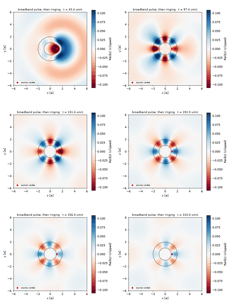
이번 질문: 어떤 주파수의 빛이 남고, 얼마나 오래 남으며, 그 답을 어떻게 검증할까요? 아래 측정은 2D Ez·손실 없는 고립 고리의 결과입니다. 도파로와의 결합 손실이나 3D 소자의 Q를 포함하지 않습니다.
English summary
- What: post 11 measured how much a dipole emits between two mirrors. On a chip the trap is a dielectric ring. This post asks the first questions about any resonator: at which frequencies does it trap light, for how long (Q), how far apart are the resonances (FSR), and what does each trapped mode look like. Official
ring.py(Harminv on the ringing field), one narrow-band run per mode, and officialsolve-cw.py(the same mode solved in the frequency domain). -
Result: a broadband pulse in the band 0.10–0.20 excites three Ez modes; at the official resolution 10 Harminv gives f = 0.1181 / 0.1472 / 0.1753 with Q = 81 / 317 / 1675 (tutorial: 0.1181 / 0.1472 / 0.1752, Q 81 / 316 / 1677). The frequencies move by less than 0.3% between resolution 10 and 30; the Q of the sharpest mode goes 1675 → 2132 → 1610, not monotonically. The spacing 0.0292 / 0.0283 matches 1/(n_g L) with n_g = 3.69, and the three modes carry m = 3, 4, 5 wavelengths around the ring. solve_cwreproduces the time-domain DFT of the f = 0.118 mode to 0.40% relative L2 (Ez correlation 0.99998) after a complex scale factor. - Takeaway: Harminv turns 300 time units of ringing into frequencies and Q without waiting for the field to decay, but Q converges much more slowly with resolution than the frequency does. One mode at a time needs a source as narrow as the mode. The frequency-domain solver and the time-domain pulse are two routes to the same steady state, and agreeing to a percent is what “the same mode” means.
- Code: full script at the bottom, ~4 min (mpirun -np 4).
공진기는 어디에 쓰일까요?
11편의 금속 상자는 구멍 하나로 Q를 조절했다. 칩 위에서는 금속 상자를 쓰지 않는다. 유전체 도파로를 고리로 말면 빛이 전반사로 돌면서 갇히고, 05편에서 본 굽힘 방사가 유일한 손실이 된다. 이 고리에 펄스를 넣으면 어떤 주파수가 남는가, 얼마나 오래 남는가, 남은 주파수들은 얼마나 떨어져 있는가. 그리고 그 답을 어떻게 재는가. 시간영역에서 울림을 분해하는 Harminv와, 주파수 영역에서 정상상태를 직접 푸는 solve_cw 두 가지로 재고 서로 맞는지 본다.
어디에 쓰이는가
고리 공진기는 실리콘 포토닉스에서 가장 많이 쓰는 부품이다. 공진 주파수, Q, FSR 세 숫자가 그대로 소자 사양이 된다.
| 응용 | 이 글의 어떤 것을 쓰는가 | 그 다음에 필요한 것 | |—|—|—| | 파장 필터, add-drop 다중화기(WDM), ring 변조기 | 공진 주파수와 FSR(채널 간격), Q(선폭 = 통과 대역) | 30편 GDS ring | | 바이오·가스 센서 | 공진 이동 Δf를 선폭 f/Q로 나눈 것이 검출 한계 | 13편 디스크 공진기 | | microring·microdisk 레이저, 주파수 빗(comb) | Q와 모드 부피(threshold), FSR(빗 간격) | 22편 비선형 | | 모든 공진 구조의 측정 절차 | Harminv로 f·Q, 좁은 대역으로 모드 하나, solve_cw로 정상상태 | 26편 photonic crystal cavity |
2. 결과를 예측해 보기
해상도를 10 → 20 → 30으로 높이면 주파수와 Q가 함께 매끄럽게 수렴할까요? 먼저 골라보세요.
예측 확인하기
두 번째입니다. 세 번째 모드의 주파수는 0.17525 → 0.17564 → 0.17572지만, Q는 1675 → 2132 → 1610입니다. Q는 작은 방사 손실을 재므로 경계를 격자로 표현하는 방식에 더 민감합니다. 뒤에서 이 차이를 실제 표로 확인합니다.
3. 원리 이해하기
고리를 한 바퀴 돌아온 파동이 같은 위상으로 만나면 보강됩니다. 그래서 아무 주파수나 남는 것이 아니라, 둘레에 맞는 공진 주파수만 남습니다. Q는 그 울림이 얼마나 천천히 사라지는지, FSR은 이웃한 공진 주파수가 얼마나 떨어져 있는지를 말합니다.
Harminv는 source가 꺼진 뒤 한 점에 남는 신호에서 주파수와 감쇠율을 함께 찾습니다. Q가 크다고 감쇠가 끝날 때까지 기다릴 필요는 없지만, 추정 오차를 확인해야 합니다. 양의 Q·관측 대역 안의 모드와 error < f/(2Q)가 기본 조건이며, 이 글의 세 모드는 error가 그 기준의 2% 아래입니다.
공진 식·기호와 정량 예측 자세히 보기
고리를 한 바퀴 돈 빛의 위상이 자기 자신과 맞을 때만 보강된다. 둘레 $L=2\pi R_{\mathrm{mid}}$에 파장이 정수 $m$개 들어가는 조건이 공진이고, 이웃한 $m$ 사이의 주파수 간격이 FSR이다. 군굴절률 $n_g$는 분산을 포함한 값이라 재료 굴절률과 다르다. 손실이 굽힘 방사뿐이면 주파수가 높을수록 빛이 고리 안쪽에 더 단단히 갇혀 Q가 커진다.
\[m\,\lambda_m = n_{\mathrm{eff}}L,\qquad \mathrm{FSR}=f_{m+1}-f_m\approx\frac{1}{n_g L},\qquad Q=\frac{f}{\Delta f}=\frac{\mathrm{Re}\,\omega}{-2\,\mathrm{Im}\,\omega}\]Harminv는 source가 꺼진 뒤 한 점에서 기록한 field를 감쇠 사인파의 합 $\sum_k a_k e^{-i\omega_k t}$로 분해한다. 복소 $\omega_k$의 실수부가 공진 주파수, 허수부가 감쇠율이고 둘의 비가 Q다. 수명이 수천 time unit인 모드도 300 time unit의 기록으로 잡히지만, 각 모드에 붙는 error가 허수부보다 작아야 그 Q를 믿을 수 있다.
주파수 영역 solver는 같은 문제를 다르게 푼다. 연속파 source를 켜고 $\nabla\times\nabla\times\mathbf E-\omega^2\varepsilon\mathbf E=i\omega\mathbf J$를 반복법(BiCGSTAB-L)으로 풀어 정상상태를 바로 얻는다. 시간영역의 펄스 + DFT와 같은 모드를 주어야 하지만 source 정규화와 전체 위상이 다르므로 복소 상수 하나를 맞춘 뒤 비교한다.
| 기호 | 뜻 | 코드 변수 |
|---|---|---|
| $R$, $w$, $n$ | 안쪽 반지름 1, 폭 1, 굴절률 3.4 (단위 a = 1 µm) | R, W, N_RING |
| $L$ | 평균 둘레 $2\pi(R+w/2)$ = 9.42 | L_RING |
| $f_{\mathrm{cen}}$, $df$ | 광대역 펄스 0.15 ± 0.05 | FCEN, DF |
| $m$ | 방위 차수(둘레의 파장 수) | m_az |
| $Q$, error | Harminv 출력 | h.modes[k].Q, .err |
| tol | solve_cw 반복 종료 기준 | TOLS |
| $\alpha$ | CW와 DFT를 맞추는 복소 상수 | alpha |
가정과 유효 범위: 2D Ez, 손실 없는 유전체, 단위 a = 1 µm(공진 파장 5.7~8.5 µm). 통신 파장으로 옮기려면 모든 길이에 0.27을 곱한다. 고리가 도파로와 결합하지 않은 고립 고리라 Q는 굽힘 방사만 반영한다.
결과 보기 전에 맞춰보기
| 물리량 | 내 예측 | 근거 |
|---|---|---|
| 대역 0.10~0.20의 모드 수 | 3 | FSR ≈ 1/(3.5 × 9.42) ≈ 0.03, 대역 0.1 |
| 공진 주파수 (res 10) | 0.118 / 0.147 / 0.175 | 공식 튜토리얼 |
| Q의 경향 | 고주파일수록 크다 | 굽힘 방사는 느슨한 구속에서 크다 |
| res 10 → 30의 주파수 변화 | 1% 안 | 파장당 20칸 이상 |
| res 10 → 30의 최고 Q 변화 | 수십 % | 노트: res 25에서 2515, 공식 res 10은 1677 |
| 방위 차수 m | 연속 정수 세 개, 3~6 사이 | $m\approx n_{\mathrm{eff}}Lf$, $n_{\mathrm{eff}}<3.4$ |
| solve_cw 오차 | tolerance를 조이면 단조 감소 | 튜토리얼 |
| CW vs 시간영역 DFT | L2 2% 안, 상관 0.999 이상 | 노트 1.2%, 0.99992 |
판정 기준: FSR이 손계산과 30% 넘게 다르면 둘레나 굴절률을 의심한다. Harminv error가 허수부보다 크면 그 Q는 보고하지 않는다. CW와 DFT가 10% 넘게 다르면 source 대칭이나 주파수가 어긋난 것이다.
4. 변수 하나 바꿔 실험하기
이번에는 Harminv가 울림을 관측하는 시간만 바꿉니다. 저장소의 code/ 폴더에서 공통 helper blogfig.py와 ring_resonator.py를 함께 두고 Meep 환경에서 실행하세요. 전체 코드는 아래 참고 자료에도 있습니다. 단일 CPU 기준 약 10분이며, 원문의 4분은 4개 MPI 프로세스를 사용한 기록입니다.
OMP_NUM_THREADS=1 python ring_resonator.py
- 원본의
T_HARMINV = 300.0으로 실행해 각 모드의 f·Q·error를 기록합니다. - 이 값만
600.0으로 바꾸고 다시 실행합니다. 구조·해상도·source는 고정합니다. - 같은 주파수의 모드를 짝지어 error와
f/(2Q)를 비교합니다. 관측 시간을 늘리는 실험과 공간 해상도를 높이는 실험은 서로 다른 오차를 확인합니다.
판단 기준: 관측 시간을 늘린 뒤 주파수와 Q가 얼마나 움직였는지 직접 기록하세요. 시간이 길어졌다는 이유만으로 Q가 정확하다고 결론 내릴 수는 없습니다. 아래 수치는 원본의 300 time unit 결과이며, 600의 새 측정값은 아닙니다.
시뮬레이션 배치와 파라미터 확인하기
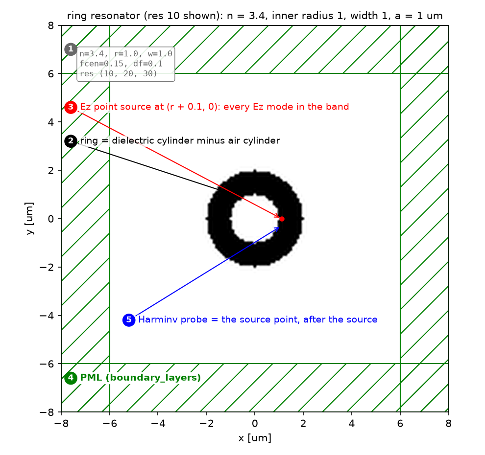
| 파라미터 | 값 | 왜 이 값인가 | 바꾸면 |
|---|---|---|---|
| 고리 | n 3.4, R 1, w 1 | 공식 ring.py | 둘레가 바뀌면 FSR이 바뀐다 |
| 펄스 | fcen 0.15, df 0.1 | 대역 0.10~0.20에 모드 셋 | 대역이 좁으면 모드를 놓친다 |
| source 위치 | (R + 0.1, 0) | 대칭축에서 비켜 모든 Ez 모드를 여기 | 축 위에 두면 odd 모드가 빠진다 |
| Harminv 창 | source 종료 후 300 | 공식 값. Q 수천까지 분해 | 너무 짧으면 error가 커진다 |
| 해상도 | 10 (공식), 20, 30 | 수렴성 | Q가 해상도에 민감(§5) |
| 모드 영상 | df 0.01, DFT at f_k | 이웃 모드(0.03 떨어짐)를 배제 | df 0.1이면 세 모드가 겹친 그림 |
| solve_cw | f 0.118, tol 1e-8/1e-10/1e-12, maxiters 10000, L 10 | 공식 solve-cw.py | L을 기본 2로 두면 수렴이 느리다 |
| CW source 대칭 | (±(R+0.1), 0)에 진폭 +1/−1, X odd | 0.118 모드의 parity | parity가 틀리면 다른 모드를 푼다 |
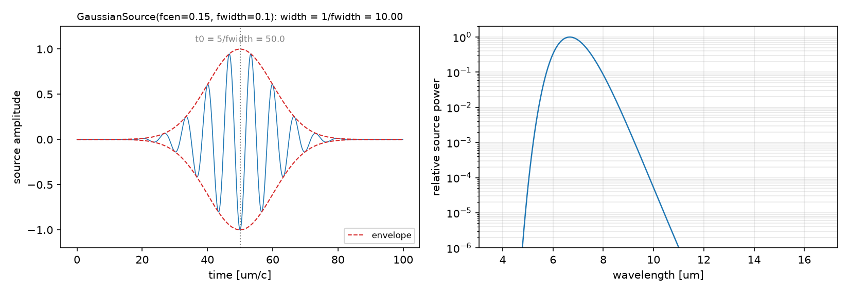
강의 노트북과의 차이: 강의 범위 밖이다. 10_sources의 0710 노트는 res 25 한 점, 0722 노트는 solve_cw tolerance 5점이었다. 이 글은 해상도 세 점(10/20/30)으로 주파수와 Q의 수렴 속도 차이를 보이고, 모드마다 좁은 대역으로 다시 돌려 방위 차수 m을 센다.
코드를 일곱 단계로 따라가기
읽는 순서: 단위·파라미터 → 재료·구조 → source → Simulation·경계 → monitor → 실행·종료 → 후처리. 이번 글의 ⑤는 flux monitor가 아니라
Harminv(한 점의 시간 신호)와solve_cw다.
① 단위와 파라미터 — 어떤 숫자를 고정하는가
N_RING, W, R = 3.4, 1.0, 1.0                # index, ring width, inner radius  [a = 1 um]
PAD, DPML = 4.0, 2.0
SXY = 2 * (R + W + PAD + DPML)              # 16 x 16
FCEN, DF = 0.15, 0.1                        # broadband pulse covering 0.10..0.20
T_HARMINV = 300.0                           # ringing window after the source (official)
L_RING = 2 * np.pi * (R + 0.5 * W)          # mean circumference, for the FSR estimate
- 무엇: 공식 값 그대로. 둘레 $L$은 FSR 손계산용.
- 왜: 실행 전에 $1/(n_g L)$로 모드 수를 어림해 두면 Harminv가 모드를 빠뜨렸는지 바로 안다.
- 틀리면: PML이 고리에 가까우면(pad 작게) 방사장이 흡수되기 전에 되돌아와 Q가 틀어진다.
② 재료와 구조 — 두 원기둥으로 고리
geometry = [mp.Cylinder(radius=R + W, material=mp.Medium(index=N_RING)),     # later objects win: outer dielectric first ...
            mp.Cylinder(radius=R)]                                             # ... then the air hole
- 무엇: 유전체 원기둥 위에 공기 원기둥을 덮어 고리를 만든다.
- 왜: Meep은 나중 객체가 앞 객체를 덮어쓴다. 순서가 반대면 유전체 원판이 된다.
- 틀리면: 11편의 금속 상자도 같은 규칙(금속 → 공기 → 구멍)이었다.
③ Source — 광대역 하나, 좁은 대역 셋, 연속파 둘
mp.Source(mp.GaussianSource(FCEN, fwidth=DF), mp.Ez, SRC_PT)                    # A: broadband, every mode in the band
mp.Source(mp.GaussianSource(f0, fwidth=0.01), mp.Ez, SRC_PT)                    # B: one mode at a time
[mp.Source(mp.ContinuousSource(F_CW), mp.Ez, mp.Vector3(R + 0.1)),             # C: continuous wave, antisymmetric pair
 mp.Source(mp.ContinuousSource(F_CW), mp.Ez, mp.Vector3(-(R + 0.1)), amplitude=-1)]
- 무엇: 목적에 따라 세 가지 source. A는 모든 모드를 한 번에, B는 하나씩, C는 정상상태.
- 왜: 모드 하나를 보려면 이웃 모드(0.03 떨어짐)가 들어오지 않는 대역(0.01)이 필요하다. Harminv의 중심 주파수를 바꾸는 것만으로는 source 스펙트럼이 바뀌지 않는다. 공식 예제 하나(ring-mode-overlap.py)가 바로 그 실수를 하고 Meep이 경고를 낸다.
- 틀리면: 연속파 source 둘의 부호가 같으면 X-even 모드를 풀게 되어 시간영역의 0.118 모드와 맞지 않는다.
④ Simulation과 경계 — 대칭과 복소 field
sim = mp.Simulation(cell_size=mp.Vector3(SXY, SXY), geometry=geometry, sources=sources, resolution=res,
                    symmetries=[mp.Mirror(mp.Y)], boundary_layers=[mp.PML(DPML)])                                   # A, B
sim = make_sim(RES_IMG, src_cw, (mp.Mirror(mp.X, phase=-1), mp.Mirror(mp.Y, phase=+1)), force_complex_fields=True)  # C
- 무엇: 사방 PML 2. A·B는 Y 거울 대칭(source가 x축 위), C는 X odd + Y even과 복소 field.
- 왜:
solve_cw는 정상상태의 진폭과 위상을 함께 주므로 복소 field가 필요하다. 대칭은 계산을 1/2, 1/4로 줄이고 모드의 parity를 고른다. - 틀리면: 11편과 같은 규칙. 위상을 전부 +1로 두면 다른 parity의 모드를 푼다.
⑤ Monitor — Harminv와 DFT, 그리고 solve_cw
h = mp.Harminv(mp.Ez, SRC_PT, FCEN, DF)                   # A: time signal at one point -> (f, Q, amp, err) per mode
sim.run(mp.after_sources(h), until_after_sources=T_HARMINV)
modes = [(m.freq, m.Q, abs(m.amp), m.err) for m in h.modes if m.Q > 0]

dft = sim.add_dft_fields([mp.Ez], f0, 0, 1, where=NONPML)  # B: steady-state field at the resonance

sim.init_sim(); sim.solve_cw(tol, MAXITERS, L_BICG)        # C: frequency-domain solve, then read the field
ez_cw = sim.get_array(vol=NONPML, component=mp.Ez)
- 무엇: Harminv는 한 점의 시간 신호를 받는 step function이다.
after_sources로 source가 꺼진 뒤부터 기록한다. B의 DFT는 공진 주파수 하나의 정상상태. C는 solve 뒤get_array로 field를 읽는다. - 왜: 공진의 세 숫자는 한 점의 시간 신호에 다 들어 있다. 공간 monitor는 모드의 모양을 볼 때만 필요하다.
- 틀리면: Harminv probe를 모드의 마디(node)에 두면 그 모드가 안 보인다. source와 같은 점을 쓰면 적어도 여기된 모드는 보인다.
⑥ 실행 — 울림 창, 감쇠 조건, 반복 종료
sim.run(mp.after_sources(h), until_after_sources=300)                                              # A: fixed window (official)
sim.run(until_after_sources=mp.stop_when_fields_decayed(50, mp.Ez, SRC_PT, 1e-6))                  # B
sim.solve_cw(tol, 10000, 10)                                                                        # C
sim.run(until_after_sources=mp.stop_when_fields_decayed(50, mp.Ez, mp.Vector3(R + 0.1523), 1e-8))   # C, time-domain comparator
- 무엇: A는 고정 창(공식). B와 C의 시간영역은 감쇠 조건. C의 solve는 tolerance와 최대 반복.
- 왜: Harminv는 감쇠가 끝나기를 기다리지 않는다. 그것이 Harminv의 존재 이유다. 반대로 DFT는 field가 다 빠져야 정확하므로 Q가 큰 모드일수록 오래 돈다(11편의 2Q/f).
- 틀리면: B에서 감쇠 기준을 느슨하게 하면 DFT에 꼬리가 남아 모드 모양에 이웃 모드가 섞인다.
⑦ 후처리 — FSR, m, 복소 정렬
fsr = np.diff(freqs); ng = 1 / (fsr.mean() * L_RING)                      # group index from the spacing
ring_vals = ez[ix, iy]                                                     # DFT field sampled on the mid-circle
m_az = int(np.argmax(np.abs(np.fft.rfft(np.real(ring_vals)))[1:]) + 1)   # dominant azimuthal order

alpha = np.vdot(ez_td, ref) / np.vdot(ez_td, ez_td)                        # best-fit complex scale
err_td = np.linalg.norm(alpha * ez_td - ref) / np.linalg.norm(ref)
- 무엇: 공진 간격에서 $n_g$를 역산하고, 고리 가운데 원 위의 field를 Fourier 변환해 $m$을 세고, CW와 DFT를 복소 상수로 맞춘 뒤 L2를 잰다.
- 왜: source 정규화(연속파 vs 펄스의 DFT)와 전체 위상은 물리가 아니다. 그것을 빼고 남는 차이가 solver의 차이다.
- 틀리면: $\alpha$ 없이 비교하면 L2가 100%를 넘고, 위상만 다른 같은 모드를 다른 모드로 읽는다.
함정: Harminv가 돌려주는 모드에는 Q가 음수이거나 error가 큰 가짜가 섞인다. Q > 0이고 대역 안에 있는 것만 남기고, error를 허수부 $f/(2Q)$와 비교한다. 이 글의 세 모드는 모두 error가 허수부의 2% 아래다.
5. 결과를 해석하기
먼저 세 번째 모드의 주파수와 Q를 나란히 읽어보세요. 해상도 10 → 30에서 주파수 변화는 0.3% 이하지만 Q는 비단조로 움직입니다. 따라서 주파수는 안정적이어도 Q의 절대값은 아직 수렴했다고 주장할 수 없습니다.
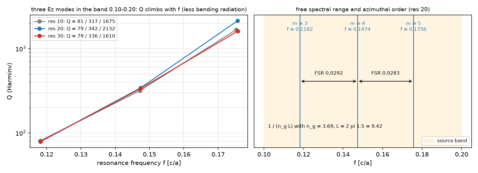
| res | $f_1$ / $Q_1$ | $f_2$ / $Q_2$ | $f_3$ / $Q_3$ |
|---|---|---|---|
| 10 (공식) | 0.11810 / 81 | 0.14716 / 317 | 0.17525 / 1675 |
| 20 | 0.11818 / 79 | 0.14736 / 342 | 0.17564 / 2132 |
| 30 | 0.11822 / 79 | 0.14740 / 336 | 0.17572 / 1610 |
| 측정 FSR | $n_g = 1/(\mathrm{FSR}\,L)$ | 고리 굴절률 |
|---|---|---|
| 0.0292 / 0.0283 | 3.69 | 3.4 |
FSR이 말하는 것: 간격 0.0292 / 0.0283에서 군굴절률 3.69를 얻습니다. 이는 재료 굴절률 3.4와 같은 양이 아닙니다. 아래 모드는 둘레에 각각 m = 3, 4, 5개의 파장이 들어갑니다.
모드 모양과 주파수 영역 교차검증 보기
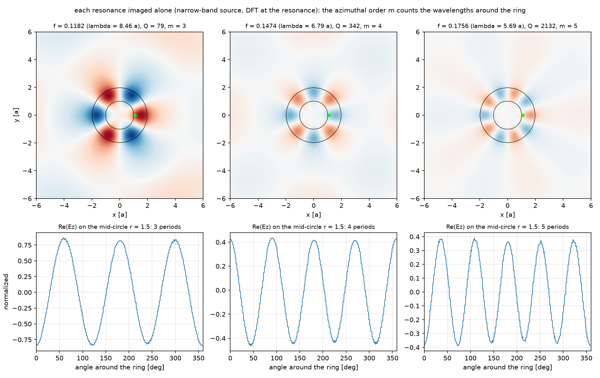
| 모드 | f | λ [a] | Q (res 20) | m | $m/(n L f)$ |
|---|---|---|---|---|---|
| 1 | 0.1182 | 8.46 | 79 | 3 | 0.79 |
| 2 | 0.1474 | 6.79 | 342 | 4 | 0.85 |
| 3 | 0.1756 | 5.69 | 2132 | 5 | 0.89 |
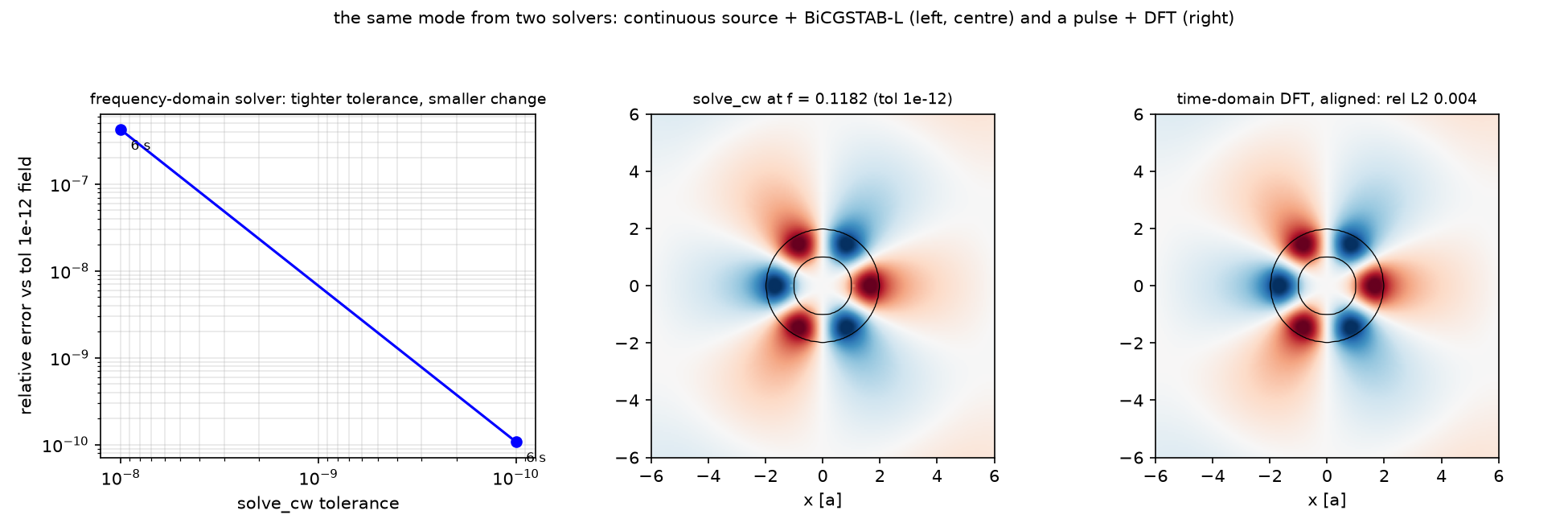
| 항목 | 값 |
|---|---|
| solve_cw tol 1e-8 / 1e-10 / 1e-12 소요 | 5 / 6 / 7 s (4 프로세스) |
| tol 1e-8, 1e-10의 상대오차 (vs 1e-12) | 4.2e-7, 1.1e-10 |
| 시간영역 DFT vs CW, 복소 정렬 후 L2 | 0.40% |
| |Ez| 상관 | 0.99998 |
| 시간영역 run 길이 (감쇠 1e-8) | 2001 time unit |
두 해법의 확인: f = 0.118 모드에서 solve_cw와 시간영역 DFT는 복소 정렬 후 상대 L2 0.40%, 진폭 상관 0.99998로 일치합니다. 이 확인이 모든 모드의 Q 수렴까지 보장하지는 않습니다.
원래의 여덟 예측·수렴성·해석 자세히 보기
예측과 비교
| 물리량 | 내 예측 (§2) | 시뮬레이션 | 판정 |
|---|---|---|---|
| 모드 수 | 3 | 3 | ✅ |
| 공진 주파수 (res 10) | 0.118 / 0.147 / 0.175 | 0.1181 / 0.1472 / 0.1753 | ✅ |
| Q 경향 | 고주파일수록 크다 | 81 → 317 → 1675 | ✅ |
| res 10→30 주파수 변화 | 1% 안 | 0.3% 이하 | ✅ |
| res 10→30 최고 Q 변화 | 수십 % | 1675 → 2132 → 1610 (비단조, ±30%) | ✅ (단조는 아님) |
| 방위 차수 m | 연속 정수, 3~6 | 3, 4, 5 | ✅ |
| solve_cw 오차 | 단조 감소 | 4.2e-7, 1.1e-10 | ✅ |
| CW vs DFT | L2 2% 안, 상관 0.999 이상 | 0.40%, 0.99998 | ✅ |
여덟 예측이 모두 방향은 맞았고, 숫자에서 두 가지를 배웠다. 첫째, Q의 해상도 의존은 단조가 아니다. 가장 날카로운 모드의 Q가 res 10에서 1675, 20에서 2132, 30에서 1610이다. 굽힘 방사는 고리 바깥 경계의 작은 누설이고, 그 누설이 격자가 경계를 어떻게 자르느냐(staircase)에 따라 달라지므로 해상도를 올려도 한 방향으로 수렴하지 않는다. 주파수는 세 해상도에서 0.3% 안이다. 둘째, $m/(n L f)$가 0.79, 0.85, 0.89로 1보다 작고 주파수가 높을수록 1에 가깝다. 모드가 고리 밖으로 새어 있어 유효 굴절률이 3.4보다 작고, 높은 모드일수록 안쪽에 갇혀 유효 굴절률이 재료값에 다가간다는 뜻이다. FSR에서 역산한 $n_g$ 3.69가 재료 굴절률보다 큰 것은 분산($n_g = n_{\mathrm{eff}} + f\,dn_{\mathrm{eff}}/df$)이고, 같은 현상의 다른 면이다. 모드 하나를 보는 run은 Q에 비례해 길어진다. Q 2132 모드는 감쇠 1e-6까지 19110 time unit이 걸렸다. Harminv가 300으로 끝내는 일을 DFT는 60배 긴 시간에 한다. solve_cw는 세 tolerance 모두 수 초였고, 시간영역 DFT와 0.4%에서 같다.
수렴성
| 변수 | 값 | 결과 | 비고 |
|---|---|---|---|
| 해상도 (Harminv) | 10 / 20 / 30 | $f_3$: 0.17525 / 0.17564 / 0.17572, $Q_3$: 1675 / 2132 / 1610 | 주파수는 20칸/파장에서 수렴, Q는 아직 |
| Harminv 창 | 300 (공식) | error ≤ 1e-5, 허수부 f/(2Q)의 2% 아래 | 창을 늘리면 error가 준다 |
| solve_cw tolerance | 1e-8 / 1e-10 / 1e-12 | 4.2e-7, 1.1e-10 | 노트: 1e-11 근처에서 비단조 |
주장할 수 있는 것 / 없는 것
- 할 수 있는 것: 이 고리(2D, n 3.4, R 1, w 1)의 대역 0.10~0.20에는 Ez 모드가 셋 있고 주파수는 해상도 10에서 이미 1% 안이다. 간격은 $n_g$ 3.69의 $1/(n_gL)$과 같다. f = 0.118 모드는 시간영역과 주파수 영역이 0.40% 안에서 같다.
- 할 수 없는 것: Q의 절대값. 해상도 30에서도 수렴하지 않았고 Harminv 창 300의 값이다. 도파로와 결합한 고리의 Q(결합 손실이 더해진다). 3D 디스크의 값. 통신 파장으로 축소했을 때의 재료 분산.
결과가 예상과 다를 때 확인할 것
| 증상 | 원인 | 고치는 법 |
|---|---|---|
| Harminv가 모드를 하나만 줌 | source 대역이 좁거나 probe가 마디 | df를 넓히고 probe를 source 점에 |
| Q가 수만, error도 큼 | 가짜 모드 | Q > 0, error < f/(2Q), 대역 안만 |
| 모드 그림에 이웃 모드가 섞임 | 모드 영상 source 대역이 FSR보다 넓음 | df < FSR/3 |
| Harminv 중심만 바꿨는데 결과 그대로 | source 스펙트럼은 안 바뀜 | source를 새로 만든다(공식 ring-mode-overlap.py의 경고) |
| solve_cw가 수렴 안 함 | L = 2, 복소 field 없음 | L = 10, force_complex_fields=True |
| CW와 DFT가 100% 다름 | 정규화·위상 미정렬, 또는 parity 다름 | 복소 상수 α로 정렬, source 부호 확인 |
| 해상도를 올렸더니 Q가 크게 변함 | 정상. Q는 느리게 수렴 | Q는 해상도 사다리와 함께 보고 |
추가 실험 아이디어
| 바꿀 것 | 예상 변화 | 확인할 수치 |
|---|---|---|
| 고리 폭 w 1 → 0.5 | 구속이 약해져 Q 감소, FSR 증가(둘레 ↓) | f, Q, FSR |
| source를 y축 위 (0, R + 0.1)에 | 기존 Y 대칭과 호환되는지 먼저 확인 | 모드 수와 source 대칭 |
| Harminv 창 300 → 1000 | error 감소, Q 안정 | error, Q |
| res 40 | Q_3 수렴 여부 | Q_3 |
| ω–2ω 겹침 (ring-mode-overlap.py) | 0.118과 0.236 모드의 공간 겹침 0.05 | 정규화 overlap |
6. 이해했는지 확인하기
- 주파수가 0.3% 안에서 안정되었는데 Q가 1675 → 2132 → 1610이라면 무엇을 보고해야 할까요?
- Harminv 관측 시간을 늘리는 것과 해상도를 높이는 것은 같은 검증일까요?
답과 이유 확인하기
- 주파수는 안정적이지만 Q의 절대값은 아직 수렴하지 않았다고 보고합니다. 사용한 해상도·관측 시간·error를 함께 제시합니다.
- 다릅니다. 관측 시간은 시간 신호에서 모드를 추정하는 오차를, 해상도는 구조와 장을 공간 격자로 표현하는 오차를 확인합니다. 작은 Harminv error만으로 공간 수렴을 보장할 수 없습니다.
7. 코드와 참고자료
공식 예제: Basics 튜토리얼의 ring resonator · Frequency-domain solver 튜토리얼 · 스크립트 ring.py · solve-cw.py.
전체 코드
code/ring_resonator.py 전체 (클릭하여 펼치기)
"""Meep Example 12 - A ring that traps light: Harminv resonances, Q, FSR, and a solve_cw cross-check.

Post 11 measured how much a dipole emits between two mirrors. On a chip the trap is a dielectric ring, and
the first questions about any resonator are: at which frequencies does it trap light, for how long (Q),
how far apart are the resonances (FSR), and what does each trapped mode look like.
  A. Official ring.py: a broadband Ez pulse inside the ring, Harminv on the ringing field after the source
     stops -> frequencies and Q of the modes in the band. Repeated at resolution 10 (official), 20, 30:
     frequencies converge fast, Q of the sharpest mode does not.
  B. Each resonance imaged alone: a narrow-band pulse at that frequency and a DFT field at the same frequency.
     The number of azimuthal lobes m is counted from the field along the ring.
  C. Official solve-cw.py: the same mode at f = 0.118 solved in the frequency domain (continuous source,
     BiCGSTAB-L), tolerance sweep, and compared with a time-domain DFT of the same mode after complex alignment.
Written to run under MPI: collective calls (run, get_array, solve_cw) on every rank, plotting on the master only.

Run:  python ring_resonator.py        (~10 min on one core, ~4 min with mpirun -np 4)
Out:  00_source.png, 01_layout.png, 02_harminv.png, 03_modes.png, 04_solve_cw.png, 05_anim_ring.gif, result.json
      (-> ../assets/12/)
"""
import json
import os
import sys
import time

import numpy as np
import matplotlib
matplotlib.use("Agg")
import matplotlib.pyplot as plt
import meep as mp

sys.path.insert(0, os.path.dirname(os.path.abspath(__file__)))
from blogfig import Label, animate_fields, annotated_layout, record_frames, source_figure   # noqa: E402

HERE = os.path.dirname(os.path.abspath(__file__))
OUT = os.path.join(HERE, "..", "assets", "12")
os.makedirs(OUT, exist_ok=True)
MASTER = mp.am_master()
t_all = time.time()


def say(*a):
    if MASTER:
        print(*a, flush=True)


# ---------------------------------------------------------------- (1) parameters (official ring.py; a = 1 um)
N_RING, W, R = 3.4, 1.0, 1.0                # index, ring width, inner radius  [a = 1 um]
PAD, DPML = 4.0, 2.0
SXY = 2 * (R + W + PAD + DPML)              # 16 x 16
FCEN, DF = 0.15, 0.1                        # broadband pulse covering 0.10..0.20
T_HARMINV = 300.0                           # ringing window after the source (official)
SRC_PT = mp.Vector3(R + 0.1)                # inside the ring, off the symmetry axes of the modes
RES_LIST = (10, 20, 30)                     # official 10, plus two finer
RES_IMG = 20                                # resolution for mode images, solve_cw, GIF
R_MID = R + 0.5 * W
L_RING = 2 * np.pi * R_MID                  # mean circumference
NONPML = mp.Volume(center=mp.Vector3(), size=mp.Vector3(SXY - 2 * DPML, SXY - 2 * DPML))
EXT = [-(0.5 * SXY - DPML), 0.5 * SXY - DPML, -(0.5 * SXY - DPML), 0.5 * SXY - DPML]

geometry = [mp.Cylinder(radius=R + W, material=mp.Medium(index=N_RING)),     # later objects win: outer dielectric first ...
            mp.Cylinder(radius=R)]                                             # ... then the air hole


def make_sim(res, sources, symmetries=(mp.Mirror(mp.Y),), **kw):
    return mp.Simulation(cell_size=mp.Vector3(SXY, SXY), geometry=geometry, sources=sources, resolution=res,
                         symmetries=list(symmetries), boundary_layers=[mp.PML(DPML)], **kw)


# ================================================================ A. Harminv at three resolutions
harm = {}
t_a = time.time()
for res in RES_LIST:
    src = [mp.Source(mp.GaussianSource(FCEN, fwidth=DF), mp.Ez, SRC_PT)]
    sim = make_sim(res, src)
    if res == RES_LIST[0]:
        annotated_layout(sim, os.path.join(OUT, "01_layout.png"), dpml=DPML, figsize=(6.6, 6.2), axis_step=2.0,
                         title="ring resonator (res 10 shown): n = 3.4, inner radius 1, width 1, a = 1 um",
                         params_text=f"n={N_RING}, r={R}, w={W}\nfcen={FCEN}, df={DF}\nres {RES_LIST}", params_xy=(-7.6, 7.0),
                         pml_xy=(-7.6, -6.6), decay_point=None,
                         labels=[Label("Ez point source at (r + 0.1, 0): every Ez mode in the band", (R + 0.1, 0.0), (-7.6, 4.6), step=3, color="red"),
                                 Label("ring = dielectric cylinder minus air cylinder", (-R_MID * 0.7, R_MID * 0.7), (-7.6, 3.2), step=2, color="black"),
                                 Label("Harminv probe = the source point, after the source", (R + 0.1, -0.3), (-5.2, -4.2), step=5, color="blue")])
    h = mp.Harminv(mp.Ez, SRC_PT, FCEN, DF)
    sim.run(mp.after_sources(h), until_after_sources=T_HARMINV)
    modes = sorted([(m.freq, m.Q, abs(m.amp), abs(m.err)) for m in h.modes if m.Q > 0 and FCEN - 0.5 * DF <= m.freq <= FCEN + 0.5 * DF])
    harm[res] = modes
    sim.reset_meep()
    say(f"A [res {res}]: " + "; ".join(f"f {f:.5f} Q {q:.0f} |amp| {a:.2e} err {e:.1e}" for f, q, a, e in modes))
modes_ref = harm[RES_IMG]
fsr = np.diff([m[0] for m in modes_ref])
ng = 1 / (np.mean(fsr) * L_RING)
say(f"A: FSR {', '.join(f'{x:.4f}' for x in fsr)} -> effective group index n_g = 1 / (FSR L) = {ng:.2f} (ring index {N_RING}); {time.time() - t_a:.0f} s")
if MASTER:
    source_figure(FCEN, DF, os.path.join(OUT, "00_source.png"), wl_scale=1.0, wl_unit="um", time_unit="um/c")

# ================================================================ B. one narrow-band run per resonance: field image + azimuthal order
imgs = []
t_b = time.time()
for f0, q0, _, _ in modes_ref:
    df0 = 0.01
    src = [mp.Source(mp.GaussianSource(f0, fwidth=df0), mp.Ez, SRC_PT)]
    sim = make_sim(RES_IMG, src)
    dft = sim.add_dft_fields([mp.Ez], f0, 0, 1, where=NONPML)
    sim.run(until_after_sources=mp.stop_when_fields_decayed(50, mp.Ez, SRC_PT, 1e-6))
    ez = sim.get_dft_array(dft, mp.Ez, 0)
    t_end = sim.meep_time()
    sim.reset_meep()
    # azimuthal order: sample the DFT field on the ring's mid-circle and count the dominant Fourier index
    nx, ny = ez.shape
    xs = np.linspace(EXT[0], EXT[1], nx); ys = np.linspace(EXT[2], EXT[3], ny)
    phis = np.linspace(0, 2 * np.pi, 720, endpoint=False)
    ix = np.clip(np.searchsorted(xs, R_MID * np.cos(phis)), 0, nx - 1); iy = np.clip(np.searchsorted(ys, R_MID * np.sin(phis)), 0, ny - 1)
    ring_vals = ez[ix, iy]
    spec = np.abs(np.fft.rfft(np.real(ring_vals)))
    m_az = int(np.argmax(spec[1:]) + 1)
    imgs.append({"f": f0, "Q": q0, "ez": ez, "m": m_az, "t_end": t_end, "ring_vals": ring_vals})
    say(f"B [f {f0:.4f}]: azimuthal order m = {m_az} (m / (n L f) = {m_az / (N_RING * L_RING * f0):.3f}); run ended at t = {t_end:.0f}")
say(f"B done in {time.time() - t_b:.0f} s")

# ================================================================ C. solve_cw at f = 0.118 vs a time-domain DFT of the same mode
F_CW = modes_ref[0][0]
sym_cw = (mp.Mirror(mp.X, phase=-1), mp.Mirror(mp.Y, phase=+1))
src_cw = [mp.Source(mp.ContinuousSource(F_CW), component=mp.Ez, center=mp.Vector3(R + 0.1)),
          mp.Source(mp.ContinuousSource(F_CW), component=mp.Ez, center=mp.Vector3(-(R + 0.1)), amplitude=-1)]
TOLS = (1e-8, 1e-10, 1e-12)
MAXITERS, L_BICG = 10000, 10
sim = make_sim(RES_IMG, src_cw, sym_cw, force_complex_fields=True)
cw = []
t_c = time.time()
for tol in TOLS:
    sim.init_sim()
    t1 = time.time()
    sim.solve_cw(tol, MAXITERS, L_BICG)
    cw.append((tol, sim.get_array(vol=NONPML, component=mp.Ez), time.time() - t1))
eps_cw = sim.get_array(vol=NONPML, component=mp.Dielectric)
sim.reset_meep()
ref = cw[-1][1]
cw_err = [float(np.linalg.norm(a - ref) / np.linalg.norm(ref)) for _, a, _ in cw[:-1]]
say("C: solve_cw " + "; ".join(f"tol {t:.0e}: {s:.0f} s" for t, _, s in cw) + " | rel error vs tightest: " + ", ".join(f"{t:.0e}: {e:.2e}" for (t, _, _), e in zip(cw[:-1], cw_err)))

src_td = [mp.Source(mp.GaussianSource(F_CW, fwidth=0.08), component=mp.Ez, center=mp.Vector3(R + 0.1)),
          mp.Source(mp.GaussianSource(F_CW, fwidth=0.08), component=mp.Ez, center=mp.Vector3(-(R + 0.1)), amplitude=-1)]
sim = make_sim(RES_IMG, src_td, sym_cw)
dft = sim.add_dft_fields([mp.Ez], F_CW, 0, 1, where=NONPML)
sim.run(until_after_sources=mp.stop_when_fields_decayed(50, mp.Ez, mp.Vector3(R + 0.1523), 1e-8))
ez_td = sim.get_dft_array(dft, mp.Ez, 0); t_td = sim.meep_time()
sim.reset_meep()
alpha = np.vdot(ez_td, ref) / np.vdot(ez_td, ez_td)          # best-fit complex scale: CW and DFT differ by amplitude and global phase
err_td = float(np.linalg.norm(alpha * ez_td - ref) / np.linalg.norm(ref))
corr = float(np.corrcoef(np.abs(ez_td).ravel(), np.abs(ref).ravel())[0, 1])
say(f"C: time-domain DFT (decay 1e-8, ended t = {t_td:.0f}) vs solve_cw after complex alignment: rel L2 {err_td:.4f}, |Ez| correlation {corr:.6f}; {time.time() - t_c:.0f} s")

# ================================================================ GIF: broadband pulse rings the resonator (monitor-free)
sim_g = make_sim(RES_IMG, [mp.Source(mp.GaussianSource(FCEN, fwidth=DF), mp.Ez, SRC_PT)])
sim_g.init_sim()
eps_g = sim_g.get_array(vol=NONPML, component=mp.Dielectric)
t0g = 5 / DF
frames, times = record_frames(sim_g, NONPML, mp.Ez, t_start=t0g - 1 / DF, t_end=t0g + 260, n_frames=80)
sim_g.reset_meep()

# ================================================================ figures (master only)
if MASTER:
    # A: Harminv results vs resolution
    fig, ax = plt.subplots(1, 2, figsize=(11, 4.0))
    cols = {10: "tab:gray", 20: "tab:blue", 30: "tab:red"}
    for j, (res, modes) in enumerate(harm.items()):
        ax[0].plot([m[0] for m in modes], [m[1] for m in modes], "o-", color=cols[res], label=f"res {res}: Q = " + " / ".join(f"{m[1]:.0f}" for m in modes))
    ax[0].set_yscale("log"); ax[0].set_xlabel("resonance frequency f [c/a]"); ax[0].set_ylabel("Q (Harminv)")
    ax[0].set_title("three Ez modes in the band 0.10-0.20: Q climbs with f (less bending radiation)", fontsize=9); ax[0].grid(alpha=0.3, which="both"); ax[0].legend(fontsize=8, loc="upper left")
    for k, (f, q, _, _) in enumerate(modes_ref):
        ax[1].axvline(f, color="tab:blue", lw=1.2); ax[1].text(f, 0.88, f"m = {imgs[k]['m']}\nf = {f:.4f}", ha="center", fontsize=8, color="tab:blue")
    ax[1].axvspan(FCEN - 0.5 * DF, FCEN + 0.5 * DF, color="orange", alpha=0.12, label="source band")
    for k in range(len(fsr)):
        ax[1].annotate("", xy=(modes_ref[k + 1][0], 0.5), xytext=(modes_ref[k][0], 0.5), arrowprops=dict(arrowstyle="<->", color="k"))
        ax[1].text(0.5 * (modes_ref[k][0] + modes_ref[k + 1][0]), 0.55, f"FSR {fsr[k]:.4f}", ha="center", fontsize=8)
    ax[1].text(0.102, 0.15, f"1 / (n_g L) with n_g = {ng:.2f}, L = 2 pi {R_MID} = {L_RING:.2f}", fontsize=8)
    ax[1].set_xlim(0.095, 0.205); ax[1].set_ylim(0, 1); ax[1].set_yticks([]); ax[1].set_xlabel("f [c/a]"); ax[1].set_title("free spectral range and azimuthal order (res 20)", fontsize=9); ax[1].legend(fontsize=8, loc="lower right")
    fig.tight_layout(); fig.savefig(os.path.join(OUT, "02_harminv.png"), dpi=150); plt.close(fig)

    # B: mode images
    fig, ax = plt.subplots(2, 3, figsize=(13, 8.2), gridspec_kw={"height_ratios": [1.6, 1]})
    for k, d in enumerate(imgs):
        ez = d["ez"]; lim = float(np.percentile(np.abs(ez), 99.5))
        ax[0, k].imshow(np.real(ez).T, extent=EXT, origin="lower", cmap="RdBu", vmin=-lim, vmax=lim, aspect="equal")
        ax[0, k].contour(np.linspace(EXT[0], EXT[1], eps_cw.shape[0]), np.linspace(EXT[2], EXT[3], eps_cw.shape[1]), eps_cw.T, levels=[0.5 * (1 + N_RING ** 2)], colors="k", linewidths=0.6)
        ax[0, k].plot(R + 0.1, 0, "o", color="lime", ms=4)
        ax[0, k].set_title(f"f = {d['f']:.4f} (lambda = {1 / d['f']:.2f} a), Q = {d['Q']:.0f}, m = {d['m']}", fontsize=9); ax[0, k].set_xlabel("x [a]")
        ax[1, k].plot(np.degrees(np.linspace(0, 2 * np.pi, 720, endpoint=False)), np.real(d["ring_vals"]) / np.max(np.abs(d["ring_vals"])), color="tab:blue", lw=1)
        ax[1, k].set_xlabel("angle around the ring [deg]"); ax[1, k].set_title(f"Re(Ez) on the mid-circle r = {R_MID}: {d['m']} periods", fontsize=9); ax[1, k].grid(alpha=0.3); ax[1, k].set_xlim(0, 360)
    ax[0, 0].set_ylabel("y [a]"); ax[1, 0].set_ylabel("normalized")
    fig.suptitle("each resonance imaged alone (narrow-band source, DFT at the resonance): the azimuthal order m counts the wavelengths around the ring", fontsize=10)
    fig.tight_layout(); fig.savefig(os.path.join(OUT, "03_modes.png"), dpi=150); plt.close(fig)

    # C: solve_cw
    fig = plt.figure(figsize=(13, 4.4))
    ax = fig.add_subplot(1, 3, 1)
    ax.loglog([t for t, _, _ in cw[:-1]], cw_err, "bo-"); ax.invert_xaxis()
    for (t, _, s), e in zip(cw[:-1], cw_err):
        ax.annotate(f"{s:.0f} s", (t, e), textcoords="offset points", xytext=(6, -12), fontsize=8)
    ax.set_xlabel("solve_cw tolerance"); ax.set_ylabel(f"relative error vs tol {TOLS[-1]:.0e} field"); ax.set_title("frequency-domain solver: tighter tolerance, smaller change", fontsize=9); ax.grid(alpha=0.3, which="both")
    lim = float(np.percentile(np.abs(ref), 99.5))
    for a, data, ttl in ((fig.add_subplot(1, 3, 2), np.real(ref), f"solve_cw at f = {F_CW:.4f} (tol {TOLS[-1]:.0e})"),
                         (fig.add_subplot(1, 3, 3), np.real(alpha * ez_td), f"time-domain DFT, aligned: rel L2 {err_td:.3f}")):
        a.imshow(data.T, extent=EXT, origin="lower", cmap="RdBu", vmin=-lim, vmax=lim, aspect="equal")
        a.contour(np.linspace(EXT[0], EXT[1], eps_cw.shape[0]), np.linspace(EXT[2], EXT[3], eps_cw.shape[1]), eps_cw.T, levels=[0.5 * (1 + N_RING ** 2)], colors="k", linewidths=0.6)
        a.set_title(ttl, fontsize=9); a.set_xlabel("x [a]")
    fig.suptitle("the same mode from two solvers: continuous source + BiCGSTAB-L (left, centre) and a pulse + DFT (right)", fontsize=10)
    fig.tight_layout(rect=[0, 0, 1, 0.93]); fig.savefig(os.path.join(OUT, "04_solve_cw.png"), dpi=150); plt.close(fig)

    animate_fields(frames, times, EXT, os.path.join(OUT, "05_anim_ring.gif"), eps=eps_g, figsize=(5.6, 5.0), dpi=70, clip_percentile=99.0, unit="a",
                   points=[(R + 0.1, 0, "red", "source / probe")], title="broadband pulse, then ringing", legend_loc="lower left")

    with open(os.path.join(OUT, "result.json"), "w") as f_:
        json.dump({"params": {"n": N_RING, "r": R, "w": W, "pad": PAD, "dpml": DPML, "fcen": FCEN, "df": DF, "T_harminv": T_HARMINV, "L_ring": L_RING},
                   "harminv": {str(k): [{"f": f, "Q": q, "amp": a, "err": e} for f, q, a, e in v] for k, v in harm.items()},
                   "fsr": fsr.tolist(), "n_g": float(ng),
                   "modes": [{"f": d["f"], "Q": d["Q"], "m": d["m"], "t_end": float(d["t_end"])} for d in imgs],
                   "solve_cw": {"f": F_CW, "tols": list(TOLS), "seconds": [s for _, _, s in cw], "rel_err_vs_tightest": cw_err,
                                "td_vs_cw_rel_l2": err_td, "td_vs_cw_corr": corr, "td_t_end": float(t_td)},
                   "wall_s_total": time.time() - t_all, "meep": mp.__version__, "np": mp.count_processors()}, f_, indent=2)
say(f"total {time.time() - t_all:.0f} s on {mp.count_processors()} process(es)")
§4의 발췌 코드와 달리 전체 코드에는 해상도 사다리, 모드 영상과 방위 차수 계산, solve_cw sweep, GIF, result.json 기록이 들어 있다. MPI로 돌릴 수 있게 collective 호출(run, get_array, solve_cw)은 모든 rank에서, 그림 저장은 master rank에서만 한다. 그림 helper blogfig.py는 시리즈 공통이며 같은 폴더(code/)에 있다. 전체 코드와 helper: https://github.com/jin-castle/meep-examples/blob/main/code.
실행 결과 (2026-10-23 실행, mpirun -np 4):
A [res 10]: f 0.11810 Q 81 |amp| 3.41e-03 err 1.0e-05; f 0.14716 Q 317 |amp| 2.86e-02 err 7.3e-07; f 0.17525 Q 1675 |amp| 7.21e-03 err 2.0e-07
A [res 20]: f 0.11818 Q 79 |amp| 3.51e-03 err 6.8e-06; f 0.14736 Q 342 |amp| 2.81e-02 err 1.7e-07; f 0.17564 Q 2132 |amp| 6.76e-03 err 1.4e-06
A [res 30]: f 0.11822 Q 79 |amp| 3.52e-03 err 2.6e-06; f 0.14740 Q 336 |amp| 2.82e-02 err 1.5e-07; f 0.17572 Q 1610 |amp| 6.79e-03 err 9.7e-08
A: FSR 0.0292, 0.0283 -> effective group index n_g = 1 / (FSR L) = 3.69 (ring index 3.4)
B [f 0.1182]: azimuthal order m = 3 (m / (n L f) = 0.792); run ended at t = 2101
B [f 0.1474]: azimuthal order m = 4 (m / (n L f) = 0.847); run ended at t = 5453
B [f 0.1756]: azimuthal order m = 5 (m / (n L f) = 0.888); run ended at t = 19110
C: solve_cw tol 1e-08: 5 s; tol 1e-10: 6 s; tol 1e-12: 7 s | rel error vs tightest: 1e-08: 4.24e-07, 1e-10: 1.08e-10
C: time-domain DFT (decay 1e-8, ended t = 2001) vs solve_cw after complex alignment: rel L2 0.0040, |Ez| correlation 0.999984
total ~4 min on 4 processes
재현 환경: meep 1.33.0 (MPI) · Python 3.11 · conda install -c conda-forge pymeep=*=mpi_mpich_* · 실행 mpirun -np 4 python ring_resonator.py (약 4 min (mpirun -np 4))
심화 질문: 다음 편과 연결하기
- Harminv는 300 time unit의 신호로 수명이 수천인 모드의 Q를 준다. 그것이 가능한 이유와, 그 Q를 믿어도 되는 조건(error)을 말해 보라.
- 주파수는 해상도 10에서 1% 안인데 Q는 해상도 30에서도 수렴하지 않았다. 두 양의 수렴 속도가 다른 이유를 굽힘 방사와 격자로 설명해 보라.
- 이 고리는 2D 단면이다. 실제 마이크로디스크는 축대칭 3D 구조이고 모드는 방위 차수 m을 가진다. 3D 셀을 돌리지 않고 m 하나당 2D 계산으로 끝내는 좌표계는 무엇이고, 그때 m은 어디에 들어가는가. (13편)
더 읽기
- Basics 튜토리얼: modes of a ring resonator · Frequency-domain solver · Harminv 레퍼런스 · solve_cw
- 스크립트: ring.py · solve-cw.py · ring-mode-overlap.py
- 이전 글: 11 · 두 거울 사이의 점광원 · 05편의 bend 손실: 05 · Bent waveguide와 radius trade-off · 다음 글: 13 · 회전 대칭으로 3D를 계산하기