MEEP EXAMPLES 05
빛은 직각 모서리를 얼마나 잘 돌아갈까?
날카로운 코너에서 새는 빛을 보고, 직선 도파로를 기준으로 투과·반사를 나눠 잽니다. 코너를 둥글릴 때 손실과 크기가 어떻게 바뀌는지 확인합니다.
이 글을 읽고 나면
- 투과·반사·방사로 나뉜 빛을 필드와 수치로 연결한다.
- 직선 기준 run과 입사장 빼기가 필요한 이유를 설명한다.
- 굽힘 반지름과 손실을 비교하고 수치 오차의 한계를 읽는다.
먼저 알면 좋은 것 04편의 도파로 모드와 03편의 reference run을 알면 좋습니다. 실행에는 Meep와 Python이 필요합니다.
English summary
- What: a dielectric waveguide (ε = 12, width 1) turns a sharp 90° corner. We measure how much power goes around the corner, how much comes back, and how much leaks out.
- Result: T = 0.20, R = 0.22, radiated = 0.58 at the center wavelength. Most of the light is lost at the sharp corner. Rounding it recovers the light: T = 0.91 at a bend radius of 0.35 µm and 0.99 at 0.70 µm.
- Takeaway: two-run flux normalization. A straight reference run gives the input power and the incident fields; subtracting them in the bend run leaves only the reflection. A sharp corner is not usable in a photonic circuit.
- Code: full script at the bottom, ~95 s on one core (the sharp bend alone takes 10 s).
1. 관찰 · 빛의 경로를 먼저 보기
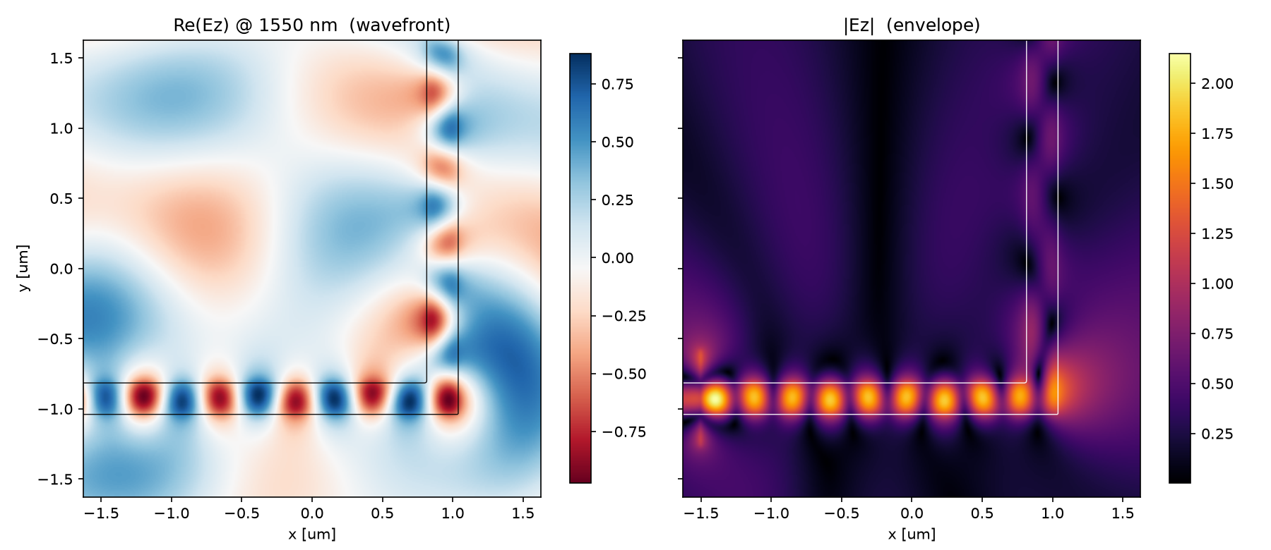
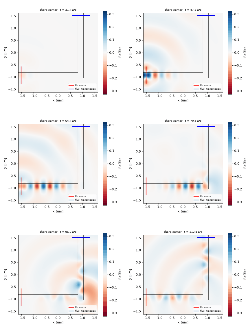
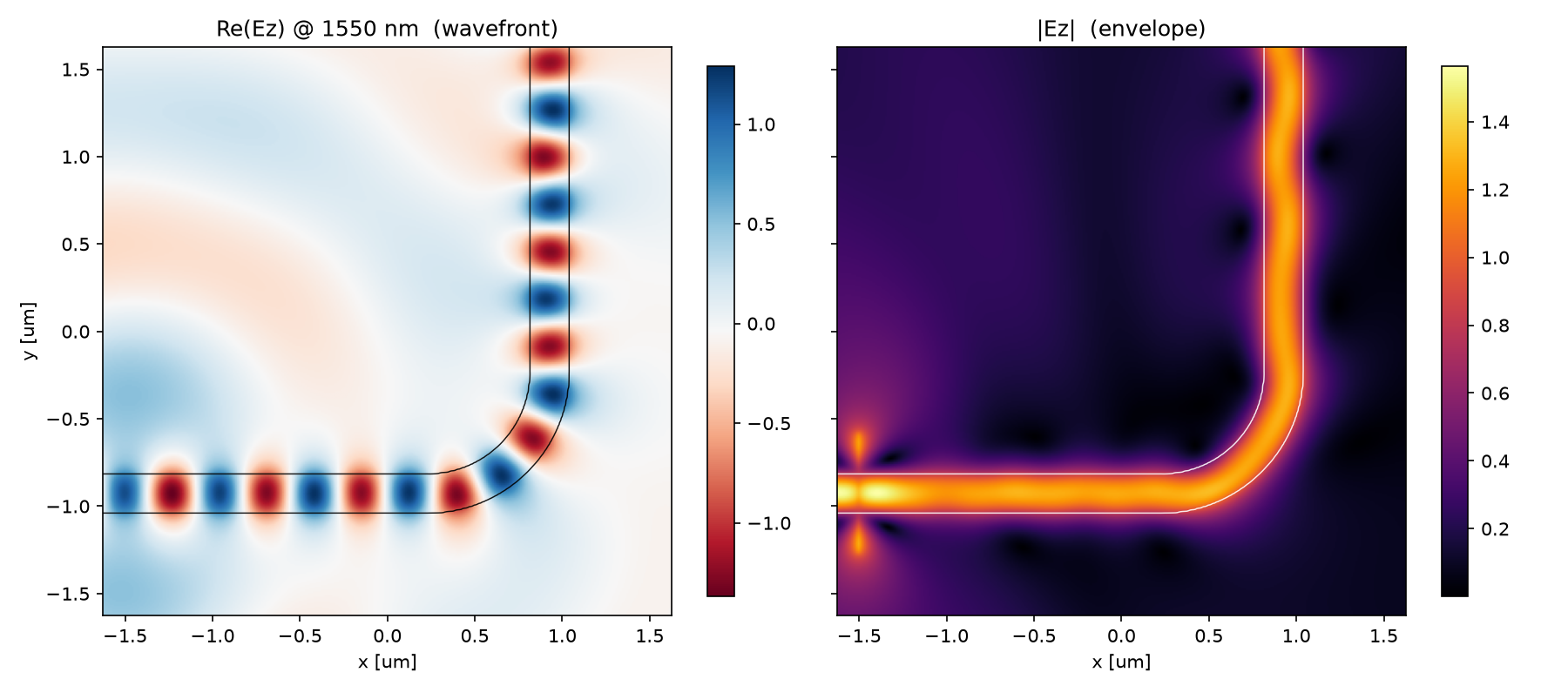
같은 폭의 도파로를 직각으로 꺾었습니다. 입력은 왼쪽, 출력은 위쪽입니다. 수평 암에서 코너까지 온 파면이 수직 암으로만 이어지는지, 주변 공기로도 퍼지는지 보세요. 필드의 밝기를 바로 투과율로 읽지 말고 뒤의 flux 측정과 연결합니다.
2. 예측 · 결과를 읽기 전에
재료가 빛을 흡수하지 않아도, 위쪽 도파로로 나가는 몫 T는 줄어들 수 있을까요?
예측의 근거 확인하기
두 번째입니다. 손실 없는 재료라는 말은 출력 도파로가 모든 power를 받는다는 뜻이 아닙니다. 입력으로 되돌아가는 반사 R과 주변 공기로 새는 방사 L도 함께 세어야 합니다. 이 구조에서는 방사가 가장 큰 몫인지 측정으로 확인합니다.
3. 원리 이해하기 · 관찰을 설명하는 방법
먼저 직선에서 기준을 만든다
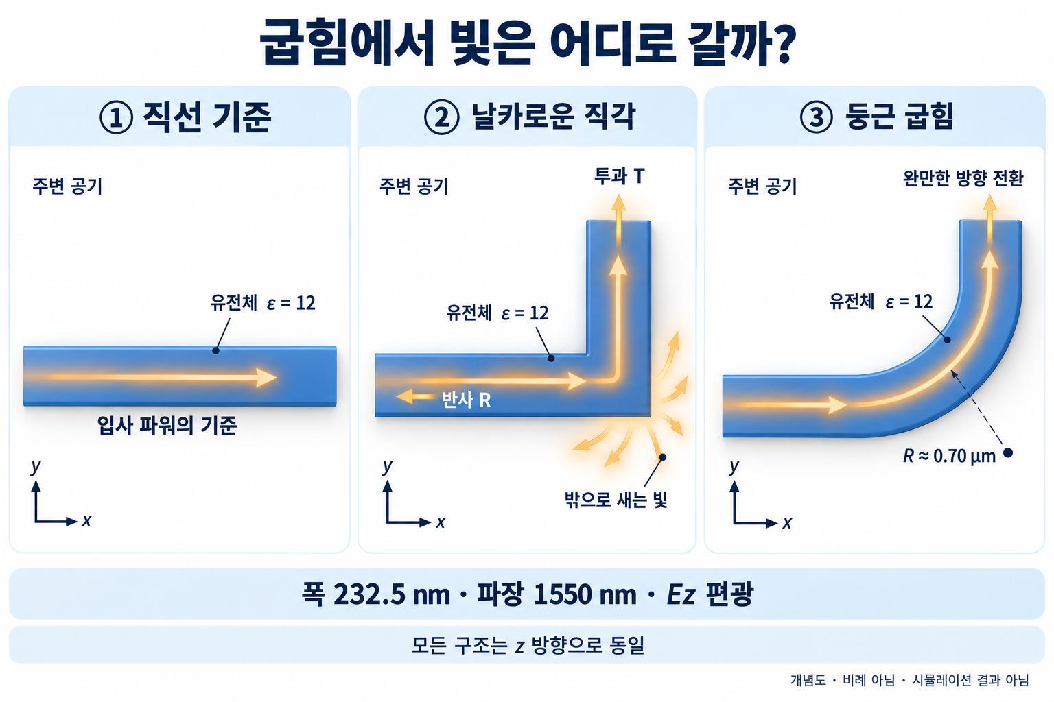
기준 run은 같은 재료·폭·source를 가진 직선 도파로입니다. 여기서 실제로 전달된 power를 입력값 P_in으로 저장하고, 반사 단면에서는 입사장의 DFT 데이터를 저장합니다. 굽힘 run에서는 같은 반사 단면에 load_minus_flux_data를 적용해 필드 수준에서 입사 성분을 뺍니다. power 숫자끼리 빼면 간섭항이 남습니다.
출력, 되돌아옴, 바깥으로 샘을 나눈다
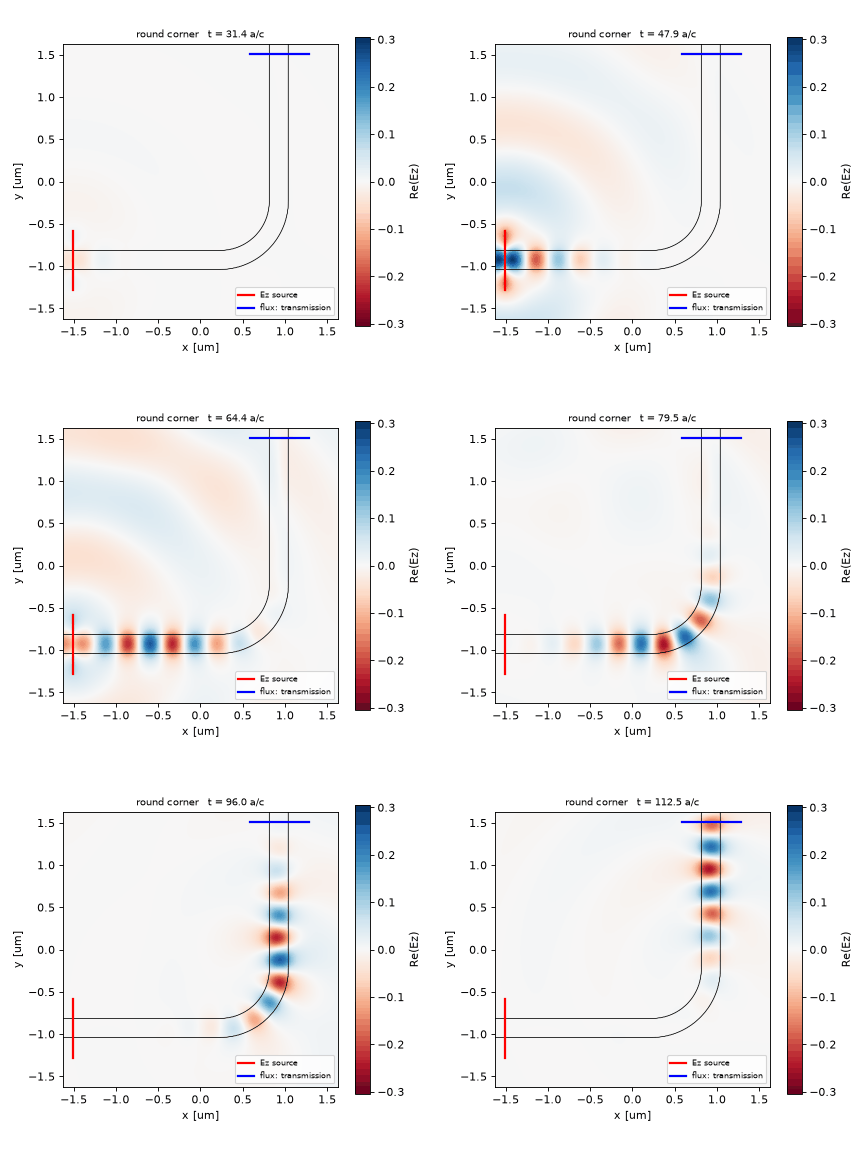
\[T=P_{\mathrm{tran}}/P_{\mathrm{in}},\qquad R=-P_{\mathrm{refl}}/P_{\mathrm{in}},\qquad L=1-T-R\]반사파는 −x로 가므로 flux가 음수이고, R 앞의 마이너스가 이를 양의 비율로 바꿉니다. 투과 monitor는 +y로 가는 빛을 가로지르는 가로선이어야 합니다. 코너가 급할수록 모드의 방향과 모양이 갑자기 바뀌어 반사·방사가 생깁니다. 둥근 코너는 그 변화를 완만하게 만듭니다.
기호·설계 가정과 예측표 자세히 보기
도파로를 따라가던 모드는 코너에서 갑자기 방향이 바뀐 도파로를 만난다. 입력 모드와 수직 암의 모드는 모양이 겹치는 부분이 작아서(mode mismatch), 겹치지 않는 부분만큼 밖으로 방사되거나 되돌아간다. 닫힌 해석해는 없고, 에너지 보존이 결과를 구속한다.
\[T=\frac{P_{\mathrm{tran}}}{P_{\mathrm{in}}},\qquad R=\frac{-P_{\mathrm{refl}}}{P_{\mathrm{in}}},\qquad T+R+L_{\mathrm{rad}}=1\]| 기호 | 뜻 | 코드 변수 |
|---|---|---|
| $P_{\mathrm{in}}$ | 직선 기준 run에서 도파로를 지나간 power | P_in |
| $P_{\mathrm{tran}}$ | bend run에서 수직 암 단면을 지나는 power | mp.get_fluxes(tran) |
| $P_{\mathrm{refl}}$ | bend run의 반사 단면 flux. 입사 성분을 뺀 값이라 뒤로 가는 power만 남고 음수 | mp.get_fluxes(refl) |
| $L_{\mathrm{rad}}$ | 코너에서 밖으로 새는 power. 직접 재지 않고 잔여로 추정 | L = 1 - T - R |
가정과 유효 범위: 2D, lossless 재료(잔여는 전부 방사), Ez 편광(면에 수직한 전기장), 공식 예제의 무차원 단위(길이 단위 a, ε = 12, 파장 6.67a). 그림에서는 a = 232.5 nm로 읽어 중심 파장을 1550 nm, 길이를 µm로 표시한다.
결과 보기 전에 맞춰보기
| 물리량 | 내 예측 | 근거 |
|---|---|---|
| T | 0.5 미만, 수십 % | 굴절률 대비가 크고(√12 ≈ 3.5) 코너가 급해 모드 겹침이 작다 |
| R | 수십 % | 코너 벽이 거울처럼 일부를 되돌린다 |
| L (방사) | 가장 큰 몫 | 코너에서 위상이 맞는 방향이 없어 대부분 밖으로 흩어진다 |
| 필드 모양 | 코너 주변 cladding으로 퍼지는 방사 lobe, 수직 암은 희미 | mode mismatch |
| T + R | 1 이하 | 에너지 보존 |
판정 기준: 이 sharp 구조의 낮은 T와 에너지 수지를 먼저 확인합니다. 작은 T + R 초과는 수치 오차일 수 있으므로 부호·정규화와 수렴성을 함께 점검합니다.
4. 직접 실행 · 변수 하나만 바꾸기
한 번만 바꿔보기: 도파로 폭
- 아래 전체 코드와 공통
blogfig.py를 같은code/폴더에 두고, 그 폴더에서python bend90.py를 실행합니다. 원본의w = 1.0결과와result.json을 별도 보관합니다. w = 1.0한 줄만w = 0.8로 바꿔 다시 실행합니다. 재료·파장·반지름 목록·해상도는 그대로 둡니다.- 두 실행의
radius_sweep에서 같은 반지름의 T·R·L을 비교합니다. T가 0.9를 넘는 첫 반지름과 sharp bend의 T도 적어 보세요.
폭이 바뀌면 모드의 구속과 코너에서의 겹침도 바뀝니다. 어느 반지름에서 차이가 커질지 먼저 예상해 보세요. 폭 0.8의 결과는 이 글에 측정되어 있지 않으며, 원본 곡선은 폭 1.0의 기준입니다. 실행할 때 출력 파일이 갱신되므로 비교용 기준 결과를 먼저 보관합니다.
계산 배치·광원·파라미터 보기
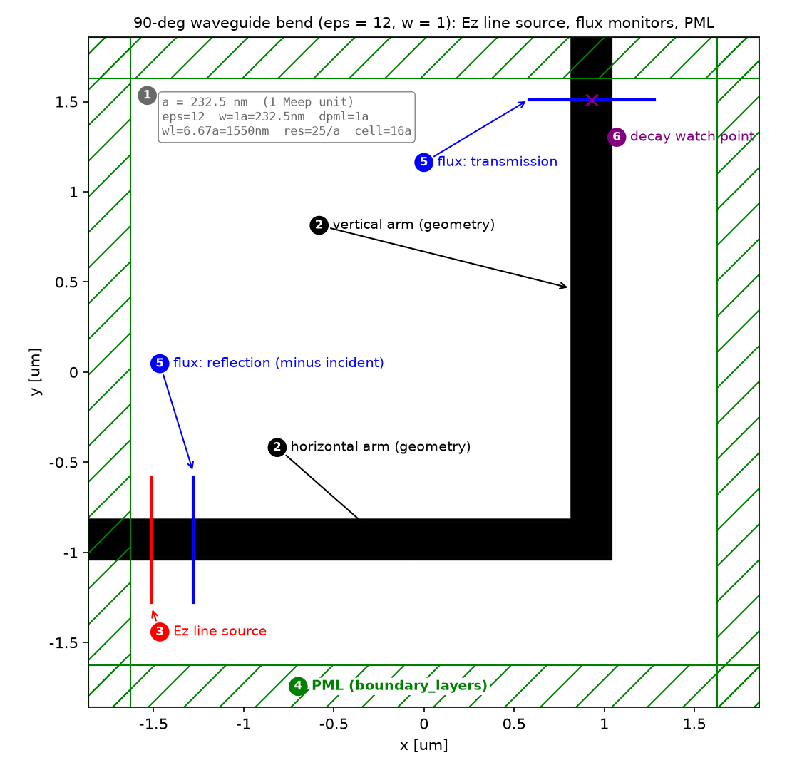
| 파라미터 | 값 | 왜 이 값인가 | 바꾸면 |
|---|---|---|---|
eps_wg, w |
12, 1 | 공식 튜토리얼 값 (n ≈ 3.46) | ε 낮추면 confinement 약해져 L ↑ |
fcen, df |
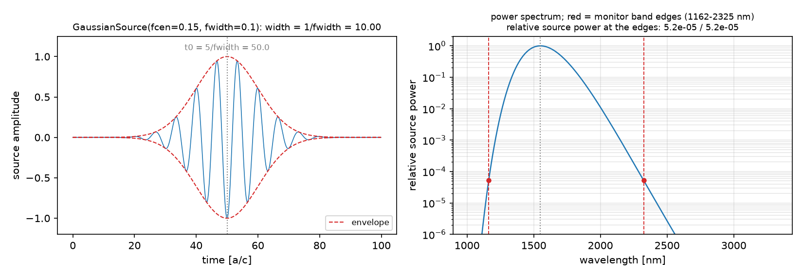
0.15, 0.1 | 파장 6.67a = 1550 nm (a = 232.5 nm). 대역 5–10a = 1160–2325 nm | 대역 가장자리는 source power가 작아 값이 튄다 |
resolution |
25 | 공식 10 → 상향. 도파로 폭 25 px, 유도 파장 48 px | 10이면 코너 형상이 거칠어 수치 변동 |
dpml |
1.0 | 파장의 1/6 이상. 양 암이 PML을 관통 | 얇으면 PML 반사가 R에 섞임 |
sx = sy |
16 | 코너 주변 방사가 PML에 닿기 전 퍼질 여유 | 좁히면 방사가 monitor에 되돌아옴 |
src_x, refl_x |
−6.5, −5.5 | source는 PML 밖 0.5, 반사 단면은 source 하류 1.0 | 반사 단면이 source 상류면 입사 성분 분리 실패 |
span |
w + 2 | core 양쪽 1a씩 evanescent tail 포함 | core 폭만 잡으면 P_in 과소 → T 과대 |
강의 노트북과의 차이: 강의 week 6은 n 3.4/1.44, 폭 0.6 µm의 곡선 bend에서 radius 0.6–3.0 µm를 훑는다. 이 글은 공식 sharp bend(ε = 12, w = 1a)를 기준값으로 두고, 같은 구조의 코너만 둥글려 radius를 훑는다.
코드 단계별 설명 보기
읽는 순서는 04편과 같다: 단위·파라미터 → 재료·구조 → source → Simulation·경계 → monitor → 실행·종료 → 후처리. 이번에는 run이 두 번이라 ⑤·⑥이 기준 run과 bend run에 한 번씩 나온다.
① 단위와 파라미터 — 어떤 숫자를 고정하는가
import numpy as np
import meep as mp

# Dimensionless units as in the official tutorial: 1 length unit = a (think 1 um).
eps_wg = 12.0            # waveguide permittivity (n = sqrt(12) = 3.46)
w = 1.0                  # waveguide width
fcen = 0.15              # center frequency -> wavelength 1/0.15 = 6.67 units
df = 0.1                 # source bandwidth
nfreq = 11               # number of frequencies in the flux monitors

resolution = 25          # pixels per unit -> width = 25 px, wavelength in the guide (1.92) = 48 px
dpml = 1.0               # PML thickness
sx = sy = 16.0           # square cell, PML included

ycen = -4.0              # y of the input (horizontal) arm
xcen = +4.0              # x of the output (vertical) arm  -> corner at (xcen, ycen)

src_x = -6.5             # source: 0.5 outside the left PML (PML edge at x = -7)
refl_x = -5.5            # reflection flux plane: downstream of the source
tran_straight_x = +6.5   # transmission plane for the straight reference run
tran_bend_y = +6.5       # transmission plane for the bend run (on the vertical arm)
span = mp.Vector3(0, w + 2)   # source / monitor line: core + 1 unit on each side (evanescent tail)
- 무엇: 공식 튜토리얼의 무차원 설정(ε = 12, w = 1, f = 0.15)과 코너 위치, source·monitor 좌표를 고정한다.
- 왜: 04편은 1 = 1 µm였지만 여기서는 길이 단위 a를 정하지 않는다. Maxwell 방정식은 scale-invariant라서 a = 1 µm로 읽으면 파장 6.67 µm, a = 0.23 µm로 읽으면 1.55 µm 결과가 그대로 된다. 이 글의 그림은 그 둘째 읽기(a = 232.5 nm)로 환산해 파장은 nm, 길이는 µm로 표시한다. 좌표는 모두 PML 경계(±7)를 기준으로 잡는다.
- 틀리면:
refl_x를 source보다 왼쪽(상류)에 두면 입사 펄스가 그 단면을 지나지 않아load_minus_flux_data가 뺄 것이 없고 R이 엉뚱해진다.
함정:
df = 0.1은 대역 5–10a로 넓다. 가장자리 파장에서는 source power가 거의 없어 T·R이 튄다. 중심 근처만 믿는다(§5).
② 재료와 구조 — 무엇이 어디에 있는가
def make_geometry(bend: bool):
    """Straight reference (bend=False) or the L-shaped bend (bend=True). Same width and material."""
    wg = mp.Medium(epsilon=eps_wg)
    if not bend:
        return [mp.Block(center=mp.Vector3(0, ycen), size=mp.Vector3(mp.inf, w), material=wg)]
    horizontal = mp.Block(center=mp.Vector3(0.5 * (-sx / 2 + xcen + w / 2), ycen),
                          size=mp.Vector3(sx / 2 + xcen + w / 2, w), material=wg)   # left PML -> corner
    vertical = mp.Block(center=mp.Vector3(xcen, 0.5 * (ycen - w / 2 + sy / 2)),
                        size=mp.Vector3(w, sy / 2 - ycen + w / 2), material=wg)     # corner -> top PML
    return [horizontal, vertical]
- 무엇: 같은 함수가 플래그 하나로 직선 기준 구조와 L자 bend 구조를 만든다. 두
Block은 코너에서 폭 w만큼 겹쳐 빈틈 없는 직각을 이룬다. - 왜: 기준 run과 bend run은 구조만 다르고 나머지는 같아야 정규화가 성립한다. 함수로 묶으면 재료·폭·좌표가 어긋날 여지가 없다. 수평 암은 왼쪽 PML을, 수직 암은 위쪽 PML을 관통해야 끝면 반사가 없다.
- 틀리면: 수평 암을 코너에서
xcen - w/2까지만 그리면 코너에 빈 사각형이 생겨 R이 커진다. 수직 암이 cell 안에서 끝나면 끝면 반사가 T에 섞인다.
②′ 둥근 코너 — 사분원 고리
r = radius
cx, cy = xcen - r, ycen + r                      # center of the quarter ring
big = r + w / 2 + 1.0
geom = [mp.Cylinder(radius=r + w / 2, center=mp.Vector3(cx, cy), material=wg),    # outer disk: waveguide
        mp.Cylinder(radius=r - w / 2, center=mp.Vector3(cx, cy), material=air),   # inner disk: air -> ring
        # keep only the lower-right quadrant (x > cx, y < cy): cover the other three with air
        mp.Block(center=mp.Vector3(cx - big / 2, cy), size=mp.Vector3(big, 2 * big), material=air),
        mp.Block(center=mp.Vector3(cx + big / 2, cy + big / 2), size=mp.Vector3(big, big), material=air)]
# the two arms are appended AFTER this list, so they are drawn on top of the air blocks
- 무엇: 반지름 r + w/2의 원판에서 r − w/2의 원판을 빼 고리를 만들고, 공기 블록으로 세 사분면을 덮어 오른쪽 아래 1/4만 남긴다. 수평 암은 x = xcen − r에서, 수직 암은 y = ycen + r에서 고리와 만난다.
- 왜: Meep의 geometry는 나중 객체가 앞 객체를 덮어쓴다. 그래서 “원판 → 공기 원판 → 공기 블록 → 암” 순서가 곧 차집합 연산이다. r = 0이면 고리가 없고 sharp 코너로 돌아간다.
- 틀리면: 암을 공기 블록보다 먼저 넣으면 블록이 암의 끝을 지운다. 공기 블록을 빠뜨리면 고리 전체가 남아 도파로가 원을 그린다.
③ Source — 빛을 어떻게 넣는가
# A plain Ez line source (not an eigenmode source), as in the official tutorial.
sources = [mp.Source(mp.GaussianSource(fcen, fwidth=df), component=mp.Ez,
                     center=mp.Vector3(src_x, ycen), size=span)]
- 무엇: 수평 암을 가로지르는 길이 3a의 세로선에서 Ez 성분 가우시안 펄스를 쏜다.
- 왜: 04편의
EigenModeSource와 달리 모드 모양을 맞추지 않은 단순 선 source다. 모드가 아닌 성분도 섞여 들어가지만, 기준 run이 실제로 도파로를 따라간 power를 재므로 그 몫은 P_in에서 빠진다. 2-run 정규화가 필요한 이유 중 하나다. - 틀리면:
component를Ey로 바꾸면 2D에서 면내 편광이 되어 다른 모드(다른 confinement)를 보게 된다.size를 core 폭만큼만 잡아도 돌아가지만 모드 결합이 나빠져 방사 잡음이 늘어난다.
④ Simulation과 경계 — 계산 상자와 PML
def make_sim(bend: bool):
    return mp.Simulation(cell_size=mp.Vector3(sx, sy), resolution=resolution,
                         boundary_layers=[mp.PML(dpml)],
                         geometry=make_geometry(bend), sources=sources)
- 무엇: 16 × 16 상자, 네 변 PML 1a, 같은 source·해상도로 구조만 바꿔
Simulation을 만드는 함수. - 왜: Meep의
Simulation객체는 run이 끝나면 필드가 남아 있어 재사용하기 어렵다. 매 run마다 새로 만드는 것이 가장 안전하고, 함수로 묶으면 두 run의 설정 일치가 보장된다. - 틀리면: 두 run에서
resolution이나cell_size가 다르면 격자 위치가 달라져load_minus_flux_data가 크기가 다른 배열을 빼려다 오류를 낸다.
⑤ Monitor — 무엇을 재는가 (기준 run)
sim = make_sim(bend=False)
refl  = sim.add_flux(fcen, df, nfreq, mp.FluxRegion(center=mp.Vector3(refl_x, ycen), size=span))
tran0 = sim.add_flux(fcen, df, nfreq, mp.FluxRegion(center=mp.Vector3(tran_straight_x, ycen), size=span))
- 무엇: 직선 구조에 반사 단면(x = −5.5)과 투과 단면(x = +6.5)을 둔다.
add_flux는 그 선을 지나는 Poynting flux를 주파수별로 누적한다. - 왜: 직선은 반사가 없으므로 투과 단면 flux가 곧 source가 도파로에 넣은 power P_in이다. 반사 단면은 이 run에서는 입사 펄스를 기록하는 용도다.
- 틀리면: 투과 단면을 PML 안에 두면 이미 흡수된 값을 재서 P_in이 작아지고 T가 과대평가된다.
⑥ 실행과 종료 조건 (기준 run)
sim.run(until_after_sources=mp.stop_when_fields_decayed(
            25, mp.Ez, mp.Vector3(tran_straight_x, ycen), 1e-6))

P_in = np.array(mp.get_fluxes(tran0))     # what actually travels down the guide = input power
refl_data = sim.get_flux_data(refl)       # incident fields at the reflection plane (to subtract later)
freqs = np.array(mp.get_flux_freqs(tran0))
- 무엇: 투과 단면 근처의 Ez가 최대값의 10⁻⁶으로 줄 때까지 돌리고, P_in과 반사 단면의 DFT 필드 데이터를 꺼내 둔다.
- 왜:
get_fluxes는 숫자(power)지만get_flux_data는 필드 자체다. 다음 run에서 필드 수준에서 빼야 간섭항까지 정확히 제거된다. power끼리 빼면 틀린다. - 틀리면: 종료가 이르면 펄스 꼬리가 단면을 다 지나지 못해 P_in이 작아지고, 다음 run의 입사 데이터도 불완전해 R에 잔여 입사 성분이 남는다.
⑤′ Monitor — 무엇을 재는가 (bend run)
sim = make_sim(bend=True)
refl = sim.add_flux(fcen, df, nfreq, mp.FluxRegion(center=mp.Vector3(refl_x, ycen), size=span))
sim.load_minus_flux_data(refl, refl_data)  # subtract the incident part -> this monitor now sees reflection only
tran = sim.add_flux(fcen, df, nfreq,
                    mp.FluxRegion(center=mp.Vector3(xcen, tran_bend_y), size=mp.Vector3(w + 2, 0)))
- 무엇: bend 구조에 같은 위치의 반사 단면을 만들고, 기준 run의 입사 데이터를 음수로 미리 채운다. 투과 단면은 수직 암 위(y = +6.5)의 가로선이다.
- 왜: 반사 단면에는 입사 펄스(오른쪽으로)와 반사 펄스(왼쪽으로)가 모두 지나간다. 입사 성분을 미리 빼 두면 run이 끝났을 때 반사 성분만 남는다.
- 틀리면: 이 줄을 빼먹으면 반사 단면에 입사 성분도 남는다. 같은 부호식으로 계산한 R은 과소평가되거나 음수가 될 수 있다.
함정: 투과 단면의
size가(w + 2, 0), 즉 가로선이다. 수직 암에서는 빛이 +y로 가므로 단면은 x 방향으로 펼쳐야 한다.span을 그대로 쓰면 세로선이 되어 빛과 평행하게 놓인다.
⑥′ 실행과 종료 조건 (bend run)
sim.run(until_after_sources=mp.stop_when_fields_decayed(
            25, mp.Ez, mp.Vector3(xcen, tran_bend_y), 1e-6))
- 무엇: 이번에는 수직 암 끝(투과 단면 위치)의 Ez가 줄어들 때까지 돌린다.
- 왜: 감시점은 빛이 마지막으로 지나가는 곳이어야 한다. bend에서는 그곳이 수직 암 끝이다.
- 틀리면: 감시점을 기준 run과 같은 (+6.5, −4)로 두면 bend 구조에서는 그곳에 도파로가 없어 필드가 금방 사라지고, 투과 펄스가 다 지나기 전에 run이 끝난다.
⑦ 후처리 — 숫자로 바꾸기
T = np.array(mp.get_fluxes(tran)) / P_in      # transmitted fraction
R = -np.array(mp.get_fluxes(refl)) / P_in     # backward flux is negative -> flip the sign
L = 1.0 - T - R                               # what is left: radiated out at the corner
ic = nfreq // 2
print(f"T = {T[ic]:.4f}, R = {R[ic]:.4f}, radiation loss = {L[ic]:.4f}")
- 무엇: 두 flux를 P_in으로 나눠 T·R을 얻고, 1에서 뺀 나머지를 방사 손실로 해석한다.
- 왜: Meep의 flux는 방향이 있다. 반사 단면의 flux는 −x 방향이라 음수로 나오므로 부호를 뒤집어야 반사된 양이 된다.
1 - T - R은 방사 monitor를 따로 두지 않았을 때의 잔여 추정이다. - 틀리면: 부호를 안 뒤집으면 R이 음수, L이 1을 넘는다.
5. 해석 · 측정값과 한계를 함께 읽기
투과가 낮아진 이유를 숫자로 확인하기
| 1550 nm의 구조 | T | R | L = 1 − T − R |
|---|---|---|---|
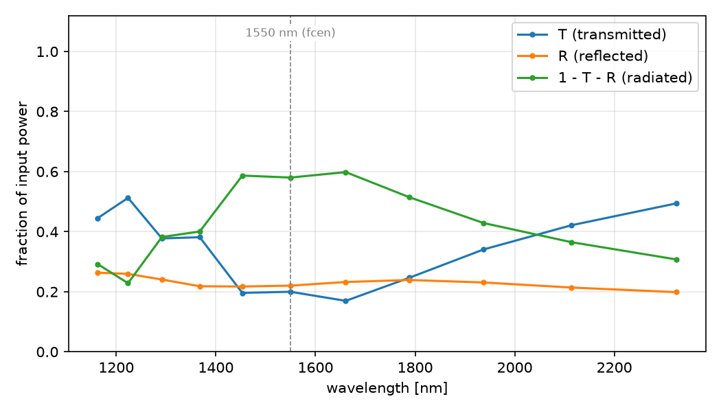
| 날카로운 코너 | 0.1997 | 0.2202 | 0.5801 |
| 반지름 3a = 0.6975 µm | 0.9859 | 0.0003 | 0.0138 |
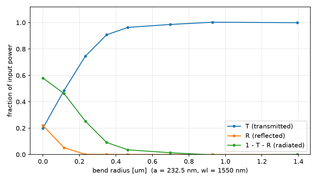
sharp bend에서는 입력의 약 20%만 위쪽 암에 도달하고 잔여 방사가 약 58%입니다. 반지름을 늘리면 반사는 약 1a에서 먼저 작아지고, 방사는 더 천천히 줄어듭니다. 이 사례의 변화가 완만해지는 구간은 1.5–2a 부근입니다.
전체 측정표·예측 비교·수렴성 기록 보기
| 물리량 | 값 @ 1550 nm (6.67a) | 비교 대상 |
|---|---|---|
| T | 0.1997 | 공식 튜토리얼도 “낮은 T” 시연 목적 |
| R | 0.2202 | — |
| L (방사, 잔여) | 0.5801 | — |
| T + R | 0.4199 | ≤ 1 성립 |
코너를 둥글리면: radius sweep
| 반지름 | µm | T | R | 방사 |
|---|---|---|---|---|
| 0 (sharp) | 0 | 0.200 | 0.220 | 0.580 |
| 0.5a | 0.12 | 0.487 | 0.052 | 0.462 |
| 1a | 0.23 | 0.746 | 0.001 | 0.253 |
| 1.5a | 0.35 | 0.907 | 0.001 | 0.092 |
| 2a | 0.47 | 0.964 | 0.000 | 0.036 |
| 3a | 0.70 | 0.986 | 0.000 | 0.014 |
| 4a | 0.93 | 1.003 | 0.000 | −0.003 |
| 6a | 1.40 | 1.000 | 0.000 | 0.000 |
반사는 반지름 1a(파장의 1/7)에서 이미 사라진다. 방사는 더 천천히 줄어 1.5a에서 10% 아래로, 3a에서 1% 대로 내려간다. 손실이 꺾이는 무릎(knee)은 1.5–2a, 즉 도파로 안 파장(1.92a)의 한 배 근처다. 그보다 큰 반지름은 면적만 늘린다. 4a에서 T가 1을 0.3% 넘는 것은 정규화 run과 bend run의 수치 오차이지 이득이 아니다.
수렴성 (sharp bend)
| resolution | dpml | T | R | 방사 | 비고 |
|---|---|---|---|---|---|
| 25 | 1.0 | 0.200 | 0.220 | 0.580 | 기준 |
| 10 | 1.0 | 0.198 | 0.229 | 0.573 | 공식 예제 해상도 |
| 40 | 1.0 | 0.189 | 0.224 | 0.587 | 해상도 1.6배 |
| 25 | 1.5 | 0.170 | 0.217 | 0.612 | PML 두껍게. source·monitor 면이 0.5a 안쪽으로 |
해상도 10에서 40까지 T는 5% 안에서 움직인다. 그런데 PML을 두껍게 하면서 source와 monitor 면을 0.5a 안쪽으로 옮기자 T가 15% 내려갔다. 코너에서 방사된 빛이 투과 단면과 PML 사이에서 어떻게 잡히느냐에 따라 값이 달라진다는 뜻이다. sharp bend의 T = 0.20은 첫째 자리까지만 의미가 있다. 둥근 bend(R ≥ 2a)는 방사가 거의 없어서 이 민감도가 사라진다.
예측과 비교
| 물리량 | 내 예측 (§2) | 시뮬레이션 | 판정 |
|---|---|---|---|
| T | 0.5 미만 | 0.20 | ✅ |
| R | 수십 % | 0.22 | ✅ |
| L | 가장 큰 몫 | 0.58 | ✅ |
| 필드 모양 | 코너 방사 lobe, 수직 암 희미 | 그림 확인 | ✅ |
| T + R | ≤ 1 | 0.42 | ✅ |
방향은 모두 맞았지만 T = 0.20이라는 값은 계산해 봐야 안다. T + R ≤ 1은 예측이 아니라 검산이다. 깨지면 물리가 아니라 코드가 틀린 것이다.
검증 체크: T + R = 0.42 ≤ 1 · source(x = −6.5)·반사 단면(−5.5)·투과 단면(y = 6.5) 모두 PML(|x|, |y| > 7) 밖 · 두 run 모두 field decay 기준 종료.
주장할 수 있는 것 / 없는 것
- 할 수 있는 것: sharp bend는 power의 절반 이상을 방사로 잃는다. 반지름을 도파로 안 파장의 한 배(1.5–2a, 0.35–0.47 µm) 이상 주면 손실이 10% 아래로 떨어지고, 3a 이상에서는 더 얻을 것이 없다.
- 할 수 없는 것: sharp bend의 T = 0.20의 둘째 자리. 해상도와 monitor 위치에 따라 0.17–0.20으로 움직인다. 3D 도파로나 다른 굴절률 대비에서의 knee 위치. 방사 monitor 없이 잔여로 추정한 방사량의 정확한 값.
증상별 점검표 보기
| 증상 | 원인 | 고치는 법 |
|---|---|---|
| 반사율 과소평가·음수 | load_minus_flux_data를 빼먹음 |
bend run에서 반사 monitor를 만든 직후 호출 |
| R이 음수 | 뒤로 가는 flux 부호를 안 뒤집음 | R = -get_fluxes(refl) / P_in |
load_minus_flux_data 배열 크기 오류 |
두 run의 resolution·cell·monitor 위치 불일치 | make_sim 같은 함수로 두 run 생성 |
| 투과 T ≈ 0 | 투과 단면이 세로선(span)으로 빛과 평행 |
수직 암에서는 size=(w+2, 0) 가로선 |
| 스펙트럼 가장자리가 튐 | 대역이 넓어 가장자리 source power ≈ 0 | df를 줄이거나 중심 ±30%만 해석 |
| R이 이상하게 큼 | 반사 단면이 source 상류, 또는 PML 얇음 | 반사 단면은 source 하류, dpml ≥ λ/6 |
6. 확인 · 두 질문에 답해보기
1. 입사장을 빼는 줄을 지우면 반사율은 어떻게 달라질까요?
설명 확인하기
반사 monitor에 입사와 반사 성분이 함께 남습니다. 이때 같은 마이너스 부호로 R을 계산하면 반사율을 과소평가하거나 음수로 얻을 수 있습니다. 이 줄은 필드를 바꾸는 source가 아니므로 투과장의 전파 자체를 바꾸지는 않습니다.
2. L = 1 − T − R가 0.58이면 방사를 정확히 58% 측정한 것일까요?
설명 확인하기
아닙니다. 여기서는 흡수 없는 모델의 잔여를 방사로 해석했습니다. monitor 위치·PML·격자 오차도 잔여에 영향을 주므로 직접 방사 flux 측정과 수렴성 확인 없이는 그 정밀도를 주장할 수 없습니다.
7. 참고 · 전체 코드와 원본 기록
아래 전체 프로그램은 원본 그대로입니다. 실행 환경과 결과 기록을 함께 확인하세요.
bend90.py (클릭해서 펼치기)
"""Meep Example 05 - Bent waveguide and the radius trade-off (two-run flux normalization).

A dielectric waveguide (eps = 12, width 1) turns a 90 degree corner.
Run 1: straight waveguide  -> input power P_in and the "incident" flux data at the reflection plane.
Run 2: bent waveguide      -> transmitted flux (vertical arm) and reflected flux (incident part subtracted).
T = P_tran / P_in,  R = -P_refl / P_in,  radiation loss = 1 - T - R.
The sharp corner (radius 0) follows the official bend-flux tutorial; then the corner is rounded
with a quarter-ring of radius R and T is swept over R to find where the loss disappears.

Run:  python bend90.py            (~3 min on one core: sharp + radius sweep + convergence)
Out:  00_source.png, 01_layout.png, 02_field.png, 03_spectrum.png, 04_radius_sweep.png,
      05_field_round.png, 06_anim_sharp.gif, 06_anim_round.gif, result.json   (-> ../assets/05/)
"""
import json
import os
import sys
import time

import numpy as np
import matplotlib
matplotlib.use("Agg")
import meep as mp

sys.path.insert(0, os.path.dirname(os.path.abspath(__file__)))
from blogfig import (Label, animate_fields, annotated_layout, field_figure, line_figure,   # noqa: E402
                     record_frames, source_figure, spectrum_figure)

OUT = os.path.join(os.path.dirname(os.path.abspath(__file__)), "..", "assets", "05")
os.makedirs(OUT, exist_ok=True)

# ---------------------------------------------------------------- (1) units & parameters
# Dimensionless units as in the official tutorial: 1 length unit = a (think 1 um).
eps_wg = 12.0            # waveguide permittivity (n = sqrt(12) = 3.46)
w = 1.0                  # waveguide width
fcen = 0.15              # center frequency -> wavelength 1/0.15 = 6.67 units
df = 0.1                 # source bandwidth
nfreq = 11               # number of frequencies in the flux monitors

# Physical reading used only for the figures: choose a so that the center wavelength is 1550 nm.
a_nm = 1550 * fcen       # = 232.5 nm per unit  -> waveguide width 233 nm, cell 3.72 um
a_um = a_nm / 1000

RESOLUTION = 25          # pixels per unit -> width = 25 px, wavelength in the guide (1.92) = 48 px
DPML = 1.0               # PML thickness
sx = sy = 16.0           # square cell, PML included

ycen = -4.0              # y of the input (horizontal) arm
xcen = +4.0              # x of the output (vertical) arm  -> corner at (xcen, ycen)
span = mp.Vector3(0, w + 2)   # source / monitor line: core + 1 unit on each side (evanescent tail)


def positions(dpml):
    """Source and monitor planes measured from the PML edge, so a thicker PML keeps them outside it."""
    edge = sx / 2 - dpml
    return {"src_x": -edge + 0.5,          # source: 0.5 outside the left PML
            "refl_x": -edge + 1.5,         # reflection flux plane: downstream of the source
            "tran_straight_x": edge - 0.5,  # transmission plane for the straight reference run
            "tran_bend_y": edge - 0.5}      # transmission plane for the bend run (on the vertical arm)


# ---------------------------------------------------------------- (2) materials & geometry
def make_geometry(bend: bool, radius: float = 0.0):
    """Straight reference (bend=False), sharp corner (radius=0) or rounded corner (radius>0).

    The rounded corner is a quarter ring: outer cylinder (waveguide) minus inner cylinder (air),
    cut down to one quadrant with air blocks; the two arms are drawn last so they stay intact.
    """
    wg = mp.Medium(epsilon=eps_wg)
    air = mp.Medium(epsilon=1.0)
    if not bend:
        return [mp.Block(center=mp.Vector3(0, ycen), size=mp.Vector3(mp.inf, w), material=wg)]
    r = radius
    cx, cy = xcen - r, ycen + r                      # center of the quarter ring
    geom = []
    if r > 0:
        big = r + w / 2 + 1.0
        geom += [mp.Cylinder(radius=r + w / 2, center=mp.Vector3(cx, cy), material=wg),
                 mp.Cylinder(radius=r - w / 2, center=mp.Vector3(cx, cy), material=air)]
        # keep only the lower-right quadrant (x > cx, y < cy)
        geom += [mp.Block(center=mp.Vector3(cx - big / 2, cy), size=mp.Vector3(big, 2 * big), material=air),
                 mp.Block(center=mp.Vector3(cx + big / 2, cy + big / 2), size=mp.Vector3(big, big), material=air)]
    # sharp corner: the arms overlap by w x w so the outer corner is filled (official geometry);
    # rounded corner: the arms stop where the ring begins
    x_end = xcen + w / 2 if r == 0 else xcen - r     # horizontal arm: left PML -> corner / ring
    horizontal = mp.Block(center=mp.Vector3(0.5 * (-sx / 2 + x_end), ycen),
                          size=mp.Vector3(sx / 2 + x_end, w), material=wg)
    y_start = ycen - w / 2 if r == 0 else ycen + r   # vertical arm: corner / ring -> top PML
    vertical = mp.Block(center=mp.Vector3(xcen, 0.5 * (y_start + sy / 2)),
                        size=mp.Vector3(w, sy / 2 - y_start), material=wg)
    return geom + [horizontal, vertical]


# ---------------------------------------------------------------- (3) source
def make_sources(dpml):
    """A plain Ez line source (not an eigenmode source), as in the official tutorial."""
    p = positions(dpml)
    return [mp.Source(mp.GaussianSource(fcen, fwidth=df), component=mp.Ez,
                      center=mp.Vector3(p["src_x"], ycen), size=span)]


# ---------------------------------------------------------------- (4) simulation & boundaries
def make_sim(bend: bool, radius=0.0, resolution=RESOLUTION, dpml=DPML):
    return mp.Simulation(cell_size=mp.Vector3(sx, sy), resolution=resolution,
                         boundary_layers=[mp.PML(dpml)],
                         geometry=make_geometry(bend, radius), sources=make_sources(dpml))


_reference = {}


def reference_run(resolution, dpml):
    """RUN 1 (cached per resolution/PML): straight guide -> P_in and the incident flux data."""
    key = (resolution, dpml)
    if key in _reference:
        return _reference[key]
    p = positions(dpml)
    sim = make_sim(bend=False, resolution=resolution, dpml=dpml)
    # ------------------------------------------------------------ (5) monitors, run 1
    refl = sim.add_flux(fcen, df, nfreq, mp.FluxRegion(center=mp.Vector3(p["refl_x"], ycen), size=span))
    tran0 = sim.add_flux(fcen, df, nfreq, mp.FluxRegion(center=mp.Vector3(p["tran_straight_x"], ycen), size=span))
    # ------------------------------------------------------------ (6) run 1 & stop condition
    sim.run(until_after_sources=mp.stop_when_fields_decayed(
                25, mp.Ez, mp.Vector3(p["tran_straight_x"], ycen), 1e-6))
    _reference[key] = {"P_in": np.array(mp.get_fluxes(tran0)),      # what actually travels down the guide
                       "refl_data": sim.get_flux_data(refl),         # incident fields at the reflection plane
                       "freqs": np.array(mp.get_flux_freqs(tran0))}
    return _reference[key]


def bend_run(radius=0.0, resolution=RESOLUTION, dpml=DPML, figures=False, field_png=None):
    """RUN 2: the bend. Returns T, R, L spectra (fractions of P_in)."""
    ref = reference_run(resolution, dpml)
    p = positions(dpml)
    sim = make_sim(bend=True, radius=radius, resolution=resolution, dpml=dpml)
    # ------------------------------------------------------------ (5) monitors, run 2
    refl = sim.add_flux(fcen, df, nfreq, mp.FluxRegion(center=mp.Vector3(p["refl_x"], ycen), size=span))
    sim.load_minus_flux_data(refl, ref["refl_data"])  # subtract the incident part -> reflection only
    tran = sim.add_flux(fcen, df, nfreq,
                        mp.FluxRegion(center=mp.Vector3(xcen, p["tran_bend_y"]), size=mp.Vector3(w + 2, 0)))
    decay_pt = (xcen, p["tran_bend_y"])
    if figures:
        annotated_layout(
            sim, os.path.join(OUT, "01_layout.png"), dpml=dpml, unit="um", axis_scale=a_um, axis_step=0.5,
            figsize=(7.5, 7.2), pml_xy=(-3.0, -sy / 2 + dpml / 2),
            params_text=(f"a = {a_nm:.1f} nm  (1 Meep unit)\n"
                         f"eps={eps_wg:g}  w={w:g}a={w*a_nm:.1f}nm  dpml={dpml:g}a\n"
                         f"wl={1/fcen:.2f}a={a_nm/fcen:.0f}nm  res={resolution}/a  cell={sx:g}a"),
            params_xy=(-6.6, 6.6), decay_point=decay_pt, decay_text_xy=(4.6, 5.6),
            title="90-deg waveguide bend (eps = 12, w = 1): Ez line source, flux monitors, PML",
            labels=[
                Label("horizontal arm (geometry)", (-1.0, ycen), (-3.5, -1.8), step=2, color="black"),
                Label("vertical arm (geometry)", (xcen - 0.5, 2.0), (-2.5, 3.5), step=2, color="black"),
                Label("Ez line source", (p["src_x"], ycen - 1.6), (-6.3, -6.2), step=3, color="red"),
                Label("flux: reflection (minus incident)", (p["refl_x"], ycen + 1.6), (-6.3, 0.2), step=5, color="blue"),
                Label("flux: transmission", (xcen - 1.5, p["tran_bend_y"]), (0.0, 5.0), step=5, color="blue"),
            ])
    want_field = figures or field_png is not None
    if want_field:
        nonpml = mp.Volume(center=mp.Vector3(), size=mp.Vector3(sx - 2 * dpml, sy - 2 * dpml))
        dft = sim.add_dft_fields([mp.Ez], fcen, 0, 1, where=nonpml)
    # ------------------------------------------------------------ (6) run 2 & stop condition
    sim.run(until_after_sources=mp.stop_when_fields_decayed(25, mp.Ez, mp.Vector3(*decay_pt), 1e-6))
    # ------------------------------------------------------------ (7) post-processing
    T = np.array(mp.get_fluxes(tran)) / ref["P_in"]      # transmitted fraction
    R = -np.array(mp.get_fluxes(refl)) / ref["P_in"]     # backward flux is negative -> flip the sign
    L = 1.0 - T - R                                      # what is left: radiated out at the corner
    if want_field:
        ez = sim.get_dft_array(dft, mp.Ez, 0)
        eps = sim.get_array(vol=nonpml, component=mp.Dielectric)
        extent_um = [v * a_um for v in (-(sx / 2 - dpml), sx / 2 - dpml, -(sy / 2 - dpml), sy / 2 - dpml)]
        field_figure(ez, extent_um, os.path.join(OUT, field_png or "02_field.png"), core_halfwidth=None,
                     eps=eps, wl=round(a_nm / fcen), wl_unit="nm", component="Ez",
                     layout="row", aspect="equal", unit="um")
    return {"T": T, "R": R, "L": L, "freqs": ref["freqs"]}


t_all = time.time()
ic = nfreq // 2

# source waveform and spectrum; the monitor band is fcen +- df/2
src_info = source_figure(fcen, df, os.path.join(OUT, "00_source.png"), mon_fcen=fcen, mon_df=df,
                         wl_scale=a_nm, wl_unit="nm", time_unit="a/c")

# ================================================================ sharp corner (official example)
t0 = time.time()
sharp = bend_run(0.0, figures=True)
wall_sharp = time.time() - t0
wl = 1 / sharp["freqs"]
print(f"sharp: T = {sharp['T'][ic]:.4f}, R = {sharp['R'][ic]:.4f}, radiation loss = {sharp['L'][ic]:.4f}  ({wall_sharp:.0f} s incl. reference)")
print(f"T over band {wl.min():.2f}-{wl.max():.2f}: {sharp['T'].min():.3f} .. {sharp['T'].max():.3f}")
spectrum_figure(wl * a_nm, {"T (transmitted)": sharp["T"], "R (reflected)": sharp["R"], "1 - T - R (radiated)": sharp["L"]},
                os.path.join(OUT, "03_spectrum.png"), unit="nm", mark=1550, mark_label="1550 nm (fcen)")

# ================================================================ radius sweep
radii = [0.0, 0.5, 1.0, 1.5, 2.0, 3.0, 4.0, 6.0]
sweep = []
for r in radii:
    if r == 0.0:
        res = sharp
    else:
        res = bend_run(r, field_png=("05_field_round.png" if r == 3.0 else None))
    sweep.append({"radius_a": r, "radius_um": r * a_um, "radius_over_wl": r * fcen,
                  "T": float(res["T"][ic]), "R": float(res["R"][ic]), "L": float(res["L"][ic])})
    print(f"radius {r:.1f} a ({r*a_um:.2f} um): T={res['T'][ic]:.4f} R={res['R'][ic]:.4f} L={res['L'][ic]:.4f}")
line_figure([s["radius_um"] for s in sweep],
            {"T (transmitted)": [s["T"] for s in sweep], "R (reflected)": [s["R"] for s in sweep],
             "1 - T - R (radiated)": [s["L"] for s in sweep]},
            os.path.join(OUT, "04_radius_sweep.png"), xlabel=f"bend radius [um]  (a = {a_nm:.1f} nm, wl = 1550 nm)")

# ================================================================ animations: sharp corner vs rounded corner (radius 3a)
# Fresh simulations with the same source; record from before the pulse peak (t0 = 5/df) until the
# pulse has gone from the source to the top monitor along the guide (distance ~ 21 a at n_eff ~ 2.5).
p = positions(DPML)
nonpml = mp.Volume(center=mp.Vector3(), size=mp.Vector3(sx - 2 * DPML, sy - 2 * DPML))
extent_um = [v * a_um for v in (-(sx / 2 - DPML), sx / 2 - DPML, -(sy / 2 - DPML), sy / 2 - DPML)]
for tag, r_anim in (("sharp", 0.0), ("round", 3.0)):
    sim_anim = make_sim(bend=True, radius=r_anim)
    sim_anim.init_sim()
    eps_anim = sim_anim.get_array(vol=nonpml, component=mp.Dielectric)
    frames, times = record_frames(sim_anim, nonpml, mp.Ez, t_start=5.0 / df - 2.0 / df,
                                  t_end=5.0 / df + 21.0 * 2.5 + 10.0, n_frames=60)
    animate_fields(frames, times, extent_um, os.path.join(OUT, f"06_anim_{tag}.gif"), eps=eps_anim,
                   lines=[((p["src_x"] * a_um, (ycen - 1.5) * a_um), (p["src_x"] * a_um, (ycen + 1.5) * a_um), "red", "Ez source"),
                          (((xcen - 1.5) * a_um, p["tran_bend_y"] * a_um), ((xcen + 1.5) * a_um, p["tran_bend_y"] * a_um), "blue", "flux: transmission")],
                   time_unit="a/c", figsize=(5.4, 4.8), title=f"{tag} corner", legend_loc="lower right")

# ================================================================ convergence (sharp corner)
convergence = [{"resolution": RESOLUTION, "dpml": DPML, "T": sweep[0]["T"], "R": sweep[0]["R"], "L": sweep[0]["L"]}]
for res_px, dpml in ((10, 1.0), (40, 1.0), (25, 1.5)):   # change one thing at a time
    t0 = time.time()
    r = bend_run(0.0, resolution=res_px, dpml=dpml)
    convergence.append({"resolution": res_px, "dpml": dpml, "T": float(r["T"][ic]), "R": float(r["R"][ic]),
                        "L": float(r["L"][ic]), "wall_s": time.time() - t0})
    print(f"convergence res={res_px} dpml={dpml}: T={r['T'][ic]:.4f} R={r['R'][ic]:.4f} L={r['L'][ic]:.4f}")

if mp.am_master():
    with open(os.path.join(OUT, "result.json"), "w") as f:
        json.dump({"T": sweep[0]["T"], "R": sweep[0]["R"], "loss": sweep[0]["L"],
                   "a_nm": a_nm, "wavelengths_a": wl.tolist(), "wavelengths_nm": (wl * a_nm).tolist(),
                   "T_spectrum": sharp["T"].tolist(), "R_spectrum": sharp["R"].tolist(),
                   "radius_sweep": sweep, "convergence": convergence, "source": src_info,
                   "wall_s_total": time.time() - t_all, "meep": mp.__version__},
                  f, indent=2)
원본 실행 로그·재현 환경 보기
§4의 발췌 코드와 달리 전체 코드에는 그림 저장·result.json 기록이 들어 있다. 그림 helper blogfig.py(annotated_layout, field_figure, spectrum_figure)는 시리즈 공통이며 같은 폴더(code/)에 있다. 전체 코드와 helper: https://github.com/jin-castle/meep-examples/blob/main/code.
실행 결과 (2026-10-23 재실행):
sharp: T = 0.1997, R = 0.2202, radiation loss = 0.5801  (10 s incl. reference)
T over band 5.00-10.00: 0.169 .. 0.512
radius 0.0 a (0.00 um): T=0.1997 R=0.2202 L=0.5801
radius 0.5 a (0.12 um): T=0.4865 R=0.0518 L=0.4617
radius 1.0 a (0.23 um): T=0.7458 R=0.0014 L=0.2528
radius 1.5 a (0.35 um): T=0.9073 R=0.0009 L=0.0918
radius 2.0 a (0.47 um): T=0.9638 R=0.0005 L=0.0358
radius 3.0 a (0.70 um): T=0.9859 R=0.0003 L=0.0138
radius 4.0 a (0.93 um): T=1.0031 R=0.0001 L=-0.0031
radius 6.0 a (1.40 um): T=0.9995 R=0.0000 L=0.0005
convergence res=10 dpml=1.0: T=0.1983 R=0.2287 L=0.5730
convergence res=40 dpml=1.0: T=0.1894 R=0.2241 L=0.5865
convergence res=25 dpml=1.5: T=0.1703 R=0.2173 L=0.6124
재현 환경: meep 1.33.0 · Python 3.11 · conda install -c conda-forge pymeep · 실행 python bend90.py (약 12 s, 단일 코어)
응용과 다음 학습 주제 보기
어디에 쓰이는가
bend 반지름은 칩 면적을 정하는 숫자다. 반지름을 두 배로 하면 고리 하나의 면적은 네 배가 되고, foundry의 설계 규칙에는 최소 반지름이 적혀 있다.
| 응용 | 이 글의 어떤 것을 쓰는가 | 그 다음에 필요한 것 |
|---|---|---|
| PIC 배선과 면적(footprint) | 반지름–손실 곡선과 knee | 09편 역설계 bend |
| ring resonator·spiral delay line | 작은 반지름의 곡률 손실이 Q와 FSR을 정한다 | 12편 고리 |
| foundry PDK의 최소 bend radius 규칙 | knee 1.5~2a가 그 규칙의 근거 | — |
| 입력 대비 출력의 모든 측정 | 2-run 정규화 | 06편 이후 전부 |