MEEP EXAMPLES 10
점광원의 빛은 어느 방향으로 나갈까?
방향별 1D 계산으로 3D 방사 패턴을 구성하고, 거울의 image가 만드는 밝고 어두운 방향을 해석합니다.
이 글을 읽고 나면
- Bloch 1D run 묶음으로 3D 패턴을 구하는 원리를 설명한다.
- flux 환산과 계산하지 않은 큰 각도의 의미를 구별한다.
- 2D 거울 모형과 3D 패턴의 비교 범위를 판단한다.
먼저 알면 좋은 것 01편 점원과 flux box · 03편 reference run
1. 먼저 보기: 점광원은 모든 방향으로 똑같이 빛날까?
01편의 2D 점원에서 한 걸음 나아가, 진동하는 축이 있는 3D 쌍극자를 봅니다. x 방향으로 진동하면 x축 방향은 어둡고, 그 축에 수직인 면에서는 고르게 빛납니다. 이를 큰 3D 셀 대신 방향별 1D 계산을 모아 재현할 수 있습니다.
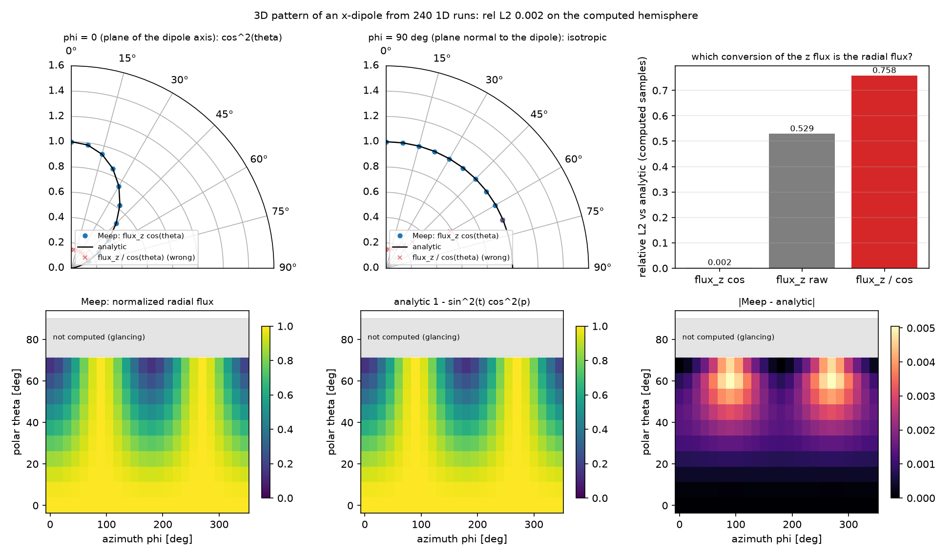
3D 패턴과 2D 그림을 구별하세요. 파트 A·C는 Bloch 1D run 묶음으로 3D Ex 쌍극자의 방향별 성분을 구합니다. 파트 B의 거울 애니메이션은 별도의 2D Ez 모델입니다. 모든 패턴 비교는 최대값으로 정규화한 모양이며 절대 방출 power나 directivity를 검증한 결과는 아닙니다.
2. 먼저 예측하기: 계산하지 않은 방향을 어떻게 읽을까?
예측과 계산 조건 비교하기
두 번째입니다. 파트 A는 sin θ > 0.95인 방향을 건너뜁니다. 거의 옆으로 진행하는 파는 z 방향 PML에 비스듬하게 들어가 흡수가 어려워집니다. 이 빈칸을 0으로 채워 해석해와 비교하면 물리적인 null과 누락된 데이터를 혼동합니다.
3. 원리 이해하기: 한 방향씩 계산하고, 거울은 image로 보기
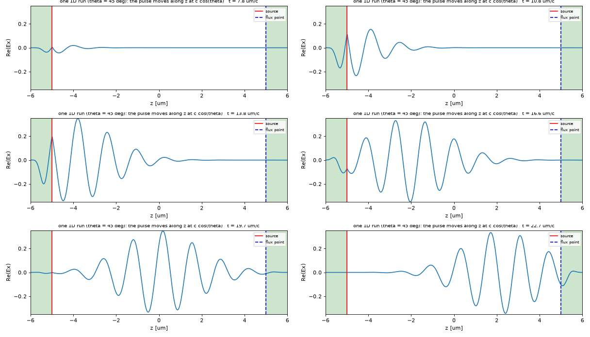
점광원의 field를 평면파 성분으로 나누면, 횡방향 파수 k_point 하나가 나가는 방향 하나에 대응합니다. 각 방향에서 z축을 따라 계산하고, 얻은 flux를 S_r = S_z cos θ로 환산한 뒤 모읍니다. θ는 +z축으로부터 잰 각도입니다.
cos θ는 단순히 z flux를 진행 방향으로 돌리는 투영만으로 정해지는 값이 아닙니다. 횡방향 파수 공간의 표본을 입체각당 power로 바꾸는 Jacobian까지 포함합니다. 원본 계산에서 곱하면 오차 0.22%, 그대로 쓰면 53%, 나누면 76%였습니다.
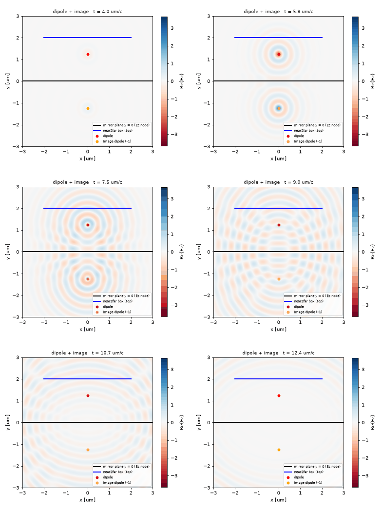
거울 옆에서는 반사된 field가 source의 field와 더해집니다. 거울에 평행한 전기 쌍극자는 거울 아래 같은 거리에 부호가 반대인 image를 놓아 설명할 수 있습니다. 둘의 경로차 2h cos θ가 방향마다 달라서 밝은 방향과 어두운 방향이 번갈아 생깁니다.
파트 B는 2D Ez·배경 n = 1.2·파장 650 nm·높이 h = 1.25 µm입니다. 반면 파트 C의 Bloch 계산은 k_point 때문에 셀 벽이 주기경계이므로, 아래쪽에 명시적인 mp.metal 블록을 넣어 거울을 만듭니다. 모든 거울은 손실 없는 PEC입니다.
4. 직접 실행하기: 거울과의 거리만 줄이기
Meep 1.33.0이 있는 환경에서 저장소의 code/ 폴더에서 원본을 실행하고 결과를 따로 보관합니다. 단일 코어의 기존 실행 기록은 약 4.3분입니다.
OMP_NUM_THREADS=1 python dipole_pattern_3d.py
높이 H만 1.25에서 0.3 µm로 바꿔 같은 명령을 실행하세요. 전체 코드의 H = 1.25를 H = 0.3으로 바꿉니다. 파트 B와 C가 공유하는 높이이므로 두 방법에 같은 변화가 적용됩니다.
05_pec_pattern.png에서 밝은 봉우리(lobe)의 개수와 각도를 원본과 비교하세요. h가 작아지면 위상차의 변화 폭도 작아져 봉우리가 줄어들 것으로 예상할 수 있습니다. 새 봉우리 위치와 오차는 실행 결과에서 읽고, 진공인 파트 A의 0.22%와 거울 계산의 오차를 섞지 마세요.
5. 결과 해석하기: 정확한 패턴에도 적용 범위가 있다
| 원본에서 비교한 것 | 상대 L2 오차 |
|---|---|
| 진공 3D 패턴, 계산한 240개 방향 | 0.22% |
| 2D near2far와 해석 array factor | 0.66% |
| 거울 위 1D Bloch와 2D, 72° 아래 | 6.4% |
| 거울 위 1D Bloch φ = 90°와 해석해, 85°까지 | 10.5% |
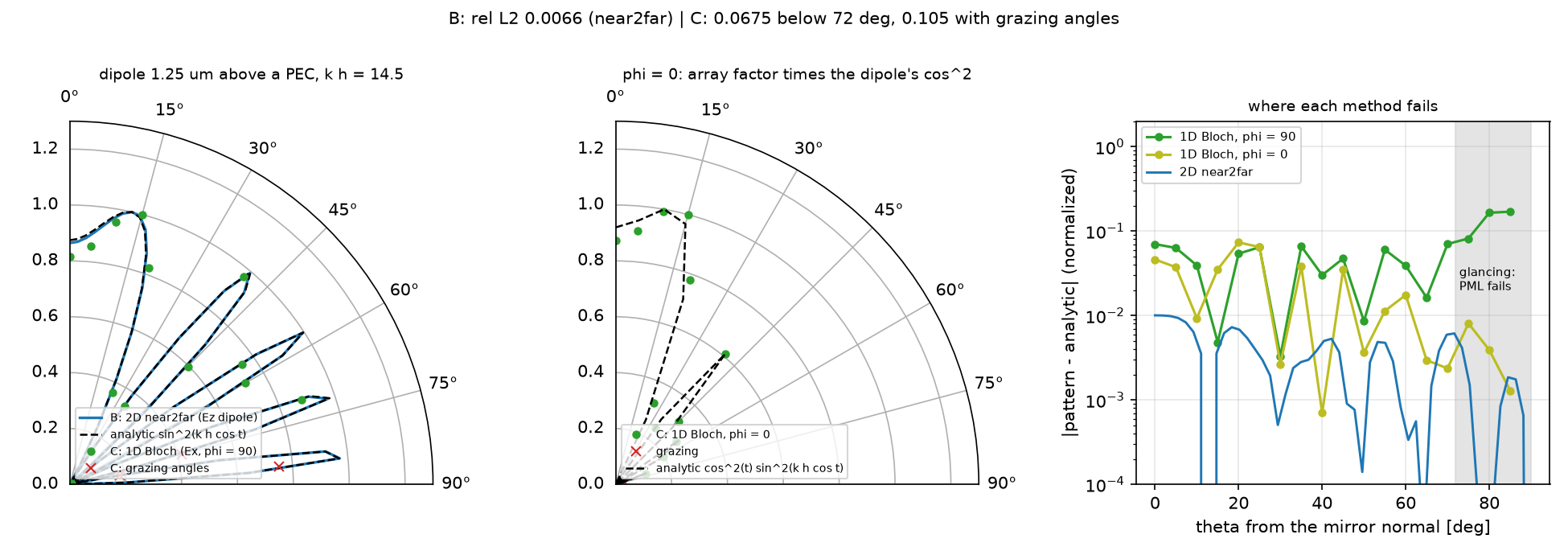
거울이 없는 경우의 0.22%를 거울 문제 전체의 정확도로 가져오면 안 됩니다. 거울 계산은 72° 아래에서도 두 방법이 6.4% 다릅니다. 원문은 거울 위치의 격자 반 칸 오차와 각도 표본 간격을 가능한 원인으로 해석하며, 여기서 두 효과를 독립적으로 검증한 것은 아닙니다.
말할 수 없는 범위. 72° 이상의 1D 방사 세기, 절대 power와 directivity, 손실 금속 거울의 응답은 검증하지 않았습니다. 2D near2far도 그 큰 각도 영역의 수렴성을 별도로 확인하지 않았습니다.
6. 이해 확인하기
- 1D run 하나로 3D 패턴 전체를 얻을 수 있나요? 필요한 반복과 환산을 설명해 보세요.
- 2D 거울 애니메이션과 3D 패턴을 비교할 때, 회색 빈칸과 6.4% 오차를 어떻게 해석해야 하나요?
두 질문의 답 확인하기
- 한 run은 한 방향의 표본입니다. 여러
k_point로 반복하고 z flux에 cos θ를 곱해 방향별 패턴을 구성합니다. - 2D Ez와 3D Ex의 적절한 단면을 정규화한 모양으로 비교합니다. 회색은 계산하지 않은 영역이고, 6.4%는 72° 아래에서도 남은 두 방법의 차이입니다. 절대 방출량의 일치를 뜻하지 않습니다.
7. 참고 자료와 전체 코드
방향별 계산 설정, 원본의 실패 사례와 상세 수치, 전체 프로그램을 아래에 보관했습니다.
English summary
TL;DR (English)
- What: post 01 left the point source radiating equally in all directions, in 2D. This post asks the 3D question twice. First, the 3D pattern of an x-polarized dipole in vacuum without a 3D cell: one 1D simulation per direction, with the direction encoded in a transverse Bloch wavevector. Second, the same dipole above a perfect-electric-conductor mirror, solved in 2D with an opposite-sign image dipole and a closed near2far box, and again with the 1D method.
- Result: 240 one-dimensional runs reproduce the dipole pattern $1-\sin^2\theta\cos^2\phi$ with 0.22% relative error on the computed hemisphere; multiplying the z flux by $\cos\theta$ is the right conversion (dividing gives 76%). Above the mirror the 2D near2far pattern matches the two-element array factor $\sin^2(kh\cos\theta)$ to 0.66% with five lobes; the 1D method agrees with it to 6.4% below 72°, and breaks down at grazing angles where the PML cannot absorb a wave travelling almost parallel to it.
- Takeaway: a 3D pattern can be bought with many cheap 1D runs, but only away from grazing angles, and the per-direction flux needs a Jacobian. An infinite mirror is never put inside a near2far box: it is replaced by an image source and a symmetry. A mirror does not just reflect; it rewrites the pattern of the source next to it.
- Code: full script at the bottom, ~4.3 min on one core.
배경·물리식·파라미터 자세히 보기
원본 §0 · 이 글에서 배우는 것
- 3D 점광원의 방사 패턴을 3D 셀 없이 얻는 법: 방향 하나 =
k_point가 다른 1D run 하나 - 1D run의 z flux를 입체각당 power로 바꾸는 환산 인자 $\cos\theta$와, 그것을 틀리게 잡으면 어떻게 보이는지
- glancing angle(72° 이상)을 공식 예제가 계산하지 않는 이유. 0으로 남은 표본은 방사 null이 아니다
- 무한 PEC 거울을 near2far box 안에 넣을 수 없을 때: 부호가 반대인 image dipole과
Mirror(Y, phase=-1) Near2FarRegion네 조각의weight가 닫힌 면의 바깥 법선이라는 것- 두 방법(2D near2far, 1D Bloch)이 같은 array factor를 내는지, 어디서 갈라지는지
전제 지식: 01편의 점원과 flux box, 03편의 reference run. 공식 예제: Near-to-far field spectra 튜토리얼의 antenna above a PEC ground plane과 dipole_in_vacuum_1D.py. 이전 글: 09 · Waveguide bend inverse design · 다음 글: 11 · 두 거울 사이의 점광원
원본 §1 · 무엇을 알고 싶은가
01편은 2D 점원이 네 면으로 25%씩 나간다는 데서 끝났다. 실제 점광원은 3D이고 축이 있다. x 방향으로 진동하는 쌍극자는 x축 방향으로는 빛을 내지 않고 그에 수직한 면에서는 고르게 낸다. 이것을 Meep으로 확인하려면 3D 셀이 필요할 것 같지만, 공식 예제는 1D run 수백 개로 같은 답을 얻는다. 왜 그것이 가능한지, 그리고 어디서 안 되는지가 첫 질문이다. 두 번째 질문은 시즌 2의 출발점이다. 점광원 옆에 거울 하나를 두면 방사 패턴은 어떻게 바뀌는가.
어디에 쓰이는가
거울 위의 쌍극자는 OLED와 LED의 발광층 그 자체다. 반사 전극 위에 놓인 발광 분자의 방사 패턴이 outcoupling의 출발점이고, 1D Bloch run 묶음은 다층 OLED의 광추출 계산에서 실제로 쓰는 방법이다.
| 응용 | 이 글의 어떤 것을 쓰는가 | 그 다음에 필요한 것 |
|---|---|---|
| OLED·LED: 반사 전극 위의 발광층 | 거울 위 쌍극자의 패턴, 1D Bloch 방법(다층으로 확장 가능) | 14편 광추출 효율 |
| 패치·모노폴 안테나(ground plane 위) | image 이론, array factor sin²(kh cosθ) | — |
| 양자점·단일광자원의 방출 방향 | 3D 쌍극자 패턴, 편광 축 | 11편 LDOS |
| 메타표면·격자의 far field | 닫힌 near2far box의 규칙 | 16편 far field |
원본 §2 · 물리 한 페이지
점광원의 field는 평면파의 합이다. 횡방향 파수 $\mathbf k_\perp=(k_x,k_y)$를 하나 고정하면 Maxwell 방정식은 z만 남은 1D 문제가 되고, 그 1D 해는 $e^{i\mathbf k_\perp\cdot\mathbf r_\perp}$를 곱한 평면파다. Meep에서 이것이 k_point다. 방향 $(\theta,\phi)$로 나가는 평면파는 $\mathbf k_\perp=f\sin\theta\,(\cos\phi,\sin\phi)$를 가지므로, 1D 셀에 쌍극자를 두고 k_point를 바꿔 가며 돌리면 run 하나가 방향 하나의 표본이 된다. 1D run이 주는 것은 그 평면파 성분의 z 방향 flux $S_z$다. 입체각당 power로 바꾸려면 $d^2k_\perp=f^2\cos\theta\,d\Omega$의 Jacobian이 들어가 $S_r=S_z\cos\theta$가 된다.
$\theta$가 90°에 가까우면 평면파가 PML과 거의 평행하게 진행한다. PML은 법선 방향으로 들어오는 파를 흡수하도록 만든 층이라 이 파는 흡수되지 않고 셀을 오간다. 공식 예제는 $|\mathbf k_\perp|>0.95f$, 즉 $\theta>71.8°$를 계산하지 않는다.
거울 위의 쌍극자는 image 이론으로 푼다. 거울에 접한 전기장은 0이어야 하므로 거울 아래 같은 거리에 부호가 반대인 쌍극자를 두면 거울면에서 두 field가 상쇄된다. 거울을 지우고 쌍극자 둘을 두는 것과 같다. 둘의 경로차가 $2h\cos\theta$이므로 방사 패턴에 array factor $4\sin^2(kh\cos\theta)$가 곱해진다. 2D Ez 쌍극자의 자체 패턴은 등방이라 2D에서는 이 인자가 패턴의 전부다.
| 기호 | 뜻 | 코드 변수 |
|---|---|---|
| $\theta,\phi$ | 극각(+z 또는 거울 법선에서), 방위각(x축에서) | POLAR, AZIM, THETA_B |
| $\mathbf k_\perp$ | 횡방향 Bloch 파수 $f\sin\theta(\cos\phi,\sin\phi)$ | k_point |
| $S_z$, $S_r$ | 1D run의 z flux, 환산한 radial flux | flux_z, radial |
| $h$ | 쌍극자와 거울 사이 거리 | H |
| $kh$ | 경로차의 위상 척도 | K_B * H |
| image | 부호 −1인 두 번째 source | amplitude=-1.0 |
가정과 유효 범위: 파트 A는 진공, 단일 주파수, Ex 편광. 파트 B는 2D Ez(거울에 접한 편광), 배경 n = 1.2, 파장 650 nm, 거울은 손실 없는 PEC. 파트 C는 3D Ex 쌍극자이고 거울은 1D 셀 아래쪽의 명시적인 mp.metal 블록이다. k_point가 있으면 셀 벽 자체는 Bloch 주기경계다. 패턴은 모두 최대값으로 정규화한 모양 비교이며 절대 power는 다루지 않는다.
결과 보기 전에 맞춰보기
| 물리량 | 내 예측 | 근거 |
|---|---|---|
| 1D run 묶음 vs 해석 패턴 (계산한 반구) | 2% 안 | 10_sources 노트의 10×12 격자에서 1.99% |
| z flux → radial flux 환산 | $\cos\theta$를 곱한다 | Jacobian $d^2k_\perp=f^2\cos\theta\,d\Omega$ |
| $\phi=90°$ 단면 | 상수(등방) | 쌍극자 축에 수직한 면 |
| 2D PEC near2far vs array factor | 1% 안 | 노트의 res 100에서 0.47% |
| 거울면 $y=0$의 $\lvert E_z\rvert$ | 0 | odd symmetry가 강제 |
| 0~90°의 lobe 수 | 5개 (12.8°, 40.7°, 57.2°, 71.0°, 83.8°) | $kh=14.5$, 극대는 $kh\cos\theta=(m+\tfrac12)\pi$ |
| 1D Bloch PEC($\phi=90°$) vs 2D near2far | 72° 아래에서 2% 안 | 같은 array factor, 쌍극자 인자는 그 면에서 1 |
| 72° 위의 1D run | 틀어진다 | PML이 평행파를 흡수하지 못한다 |
판정 기준: 계산한 반구의 상대 L2 > 5%면 환산 인자나 k_point를 의심한다. $y=0$의 $\lvert E_z\rvert$가 최대의 수 % 이상이면 symmetry 위상이 틀렸다(격자 반 칸 때문에 정확히 0은 아니다). 두 방법이 72° 아래에서 10% 이상 다르면 한쪽의 거울이나 monitor 위치를 의심한다.
원본 §3 · 시뮬레이션 설계도
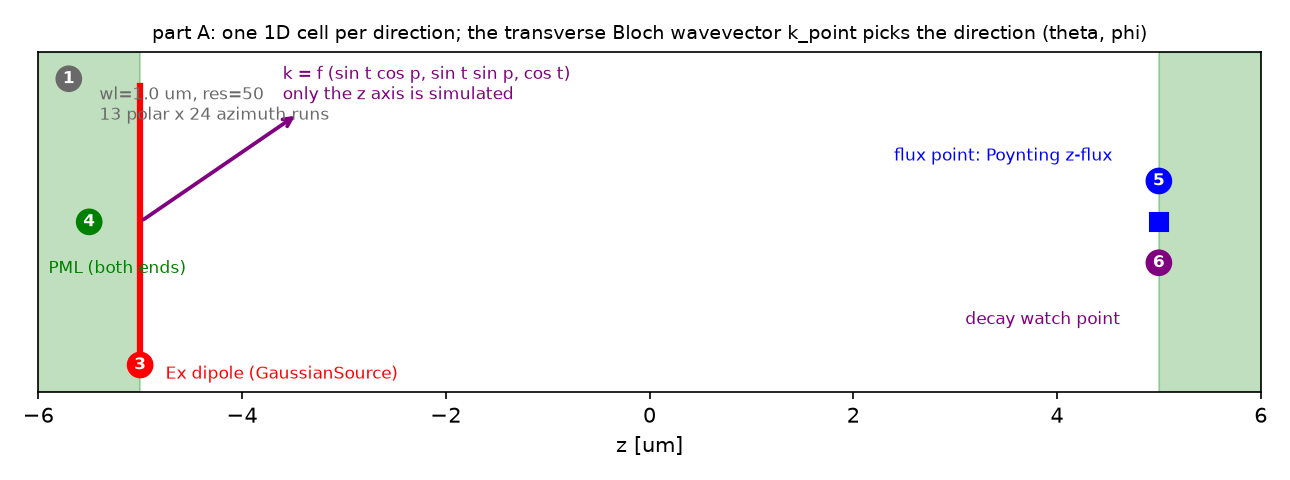
k_point로 정해지는 전파 방향이다. 동그라미 숫자는 §4의 단계 번호다.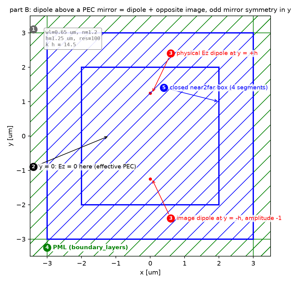
| 파라미터 | 값 | 왜 이 값인가 | 바꾸면 |
|---|---|---|---|
| A 파장, 해상도, 공기층 | 1 µm, res 50, 10 µm | 패턴은 스케일에 무관. 공식 예제 값 | 해상도는 환산 인자와 무관하다 |
| A 각도 격자 | 극각 13 × 방위각 24 | 공식 30 × 50의 축소판. 7.5°·15° 간격 | 촘촘할수록 run 수에 비례해 느려진다 |
| A glancing 한계 | $\sin\theta>0.95$ 건너뜀 | 공식 규칙. PML 평행파 | 계산하면 run이 오래 걸리고 값이 틀린다(파트 C에서 보임) |
| A 종료 | Ex 감쇠 1e-6 (25 단위 창) | 공식 예제 값 | 설정이 맞으면 run당 1초 안에 끝난다 |
A k_point |
$nf(\sin\theta\cos\phi,\ \sin\theta\sin\phi,\ \cos\theta)$ | z 성분으로 항상 $\mathbf k\neq0$ | §4 ③ |
| B 파장, n, h | 650 nm, 1.2, 1.25 µm | 공식 예제 값. $kh=14.5$ | h가 작아지면 lobe가 줄어든다 |
| B 해상도 | 100 | 노트와 같다. 파장당 83칸 | 50이면 L2가 커진다 |
| B near2far box | 반폭 2 µm | 두 쌍극자(±1.25)를 감싼다 | box가 한쪽 쌍극자만 감싸면 image 이론이 깨진다 |
| B 원거리 반지름 | 1000 λ | far field 근사 | — |
| C 셀 | metal 0.5 + h 1.25 + 공기 10 + PML 1 µm | k_point가 있으면 셀 벽은 Bloch 주기라 거울은 mp.metal 블록으로 |
벽을 거울로 믿으면 거울이 없다(§4 ④) |
| C 종료 | 고정 150 time unit | 85°의 파가 공기 10 µm(n 1.2)를 가로지르는 시간 140 | 감쇠 조건은 glancing에서 정체 |
강의 노트북과의 차이: 강의 범위 밖이다. 01편(강의 week 2)의 점광원을 3D와 거울로 확장한다. 10_sources의 두 PEC 노트가 각각 2D near2far(L2 0.47%)와 1D Bloch(상관 0.947)를 따로 다뤘는데, 이 글은 둘을 같은 축에 올려 어디서 갈라지는지 본다.
원본 코드 단계별 설명
원본 §4 · 코드 따라가기
읽는 순서: 단위·파라미터 → 재료·구조 → source → Simulation·경계 → monitor → 실행·종료 → 후처리. 파트 A·C는 1D라 ②가 없고, 파트 B는 ②가 “거울 대신 image + symmetry”다.
① 단위와 파라미터 — 어떤 숫자를 고정하는가
POLAR = np.radians(np.arange(0.0, 90.1, 7.5))      # 13 polar angles (0 = +z)
AZIM = np.radians(np.arange(0.0, 360.0, 15.0))     # 24 azimuth angles
GLANCING = 0.95                                     # skip k_perp > 0.95 f (official rule)
T_AFTER = 60.0                                      # run time after the source turns off

WL_B, N_B, H, RES_B = 0.65, 1.2, 1.25, 100          # PEC mirror part: wavelength, background index, height, resolution
K_B = 2 * np.pi * N_B / WL_B                        # k h = 14.5 sets the lobes
- 무엇: 파트 A의 각도 격자와 glancing 한계, 파트 B의 거울 문제 파라미터.
- 왜: 각도 격자는 run 수다. 13 × 24에서 glancing 3행을 빼면 240 run. $kh$는 lobe의 수와 위치를 정하므로 파장·굴절률·높이 셋을 한 묶음으로 적는다.
- 틀리면:
K_B에 배경 굴절률을 빼먹으면 array factor의 lobe가 다른 각도에 온다.
② 재료와 구조 — 거울 대신 image와 symmetry
sources_B = [mp.Source(mp.GaussianSource(FCEN_B, fwidth=FWIDTH_B), component=mp.Ez, center=mp.Vector3(0, H)),
             mp.Source(mp.GaussianSource(FCEN_B, fwidth=FWIDTH_B), component=mp.Ez, center=mp.Vector3(0, -H), amplitude=-1.0)]
symB = [mp.Mirror(mp.X), mp.Mirror(mp.Y, phase=-1)]        # odd in y -> Ez = 0 on y = 0 (the PEC plane)
- 무엇: 거울은 geometry에 없다. 부호가 반대인 두 번째 쌍극자와 y에 대한 odd mirror symmetry가 거울이다.
- 왜: 무한 PEC 판을 near2far box가 가로지를 수 없다. 두 쌍극자를 box가 감싸게 하면 변환 가정이 유지된다. symmetry는 계산을 1/4로 줄이고 $y=0$의 $E_z=0$을 정확히 강제한다.
- 틀리면:
phase=-1을 빼면 두 쌍극자가 같은 부호로 더해져 $y=0$이 node가 아니라 antinode가 되고, 패턴은 $\cos^2$ 형이 된다. Hz 편광이면 image 부호와 parity가 반대다.
③ Source — 1D 셀의 쌍극자와 k_point
def bloch_k(theta, phi, fcen, n_index=1.0):          # full wavevector of the outgoing plane wave, |k| = n f
    return mp.Vector3(n_index * fcen * np.sin(theta) * np.cos(phi), n_index * fcen * np.sin(theta) * np.sin(phi), n_index * fcen * np.cos(theta))

sim = mp.Simulation(cell_size=mp.Vector3(0, 0, sz), resolution=RES_A, k_point=bloch_k(theta, phi, fcen, n_index),   # no dimensions=1 (see below)
                    default_material=mp.Medium(index=n_index), boundary_layers=[mp.PML(thickness=DPML_A, direction=mp.Z)],
                    sources=[mp.Source(mp.GaussianSource(fcen, fwidth=fwidth), component=mp.Ex, center=mp.Vector3(0, 0, z_src), size=mp.Vector3())])
- 무엇: 셀은 z 한 줄이고 source는 그 위의 한 점이다.
k_point가 나가는 평면파의 파수 벡터 전체(횡방향 두 성분과 z 성분)를 준다. - 왜: 같은 1D 구조에서
k_point만 바꾸면 다른 방향의 평면파 성분이 된다. 3D 셀을 돌리지 않고 방향별 표본을 얻는 원리다. z 성분은 PML이 흡수하는 방향이라 물리에는 영향이 없지만, $\theta=0$에서도 $\mathbf k\neq0$이 되게 해 모든 run이 복소 field를 쓰도록 만든다. - 틀리면: 두 가지를 이 글에서 직접 겪었다.
dimensions=1을 명시하면 횡방향 k가 조용히 무시되어 flux가 각도에 무관해진다(패턴 L2 35%). z 성분 없이 $\theta=0$을 돌리면 그 run만 실수 field가 되어 power가 1/4로 나온다. 셀 크기(0, 0, sz)만으로 1D가 되므로dimensions는 쓰지 않는다.
④ Simulation과 경계 — PML의 방향과 거울
boundary_layers=[mp.PML(thickness=DPML_A, direction=mp.Z)]                     # part A: both ends of z
boundary_layers=[mp.PML(thickness=DPML_A, direction=mp.Z, side=mp.High)]       # part C: PML on top only ...
mirror = [mp.Block(center=mp.Vector3(0, 0, Z_BOT + 0.5 * DMETAL), size=mp.Vector3(mp.inf, mp.inf, DMETAL), material=mp.metal)]   # ... and a PEC block at the bottom
- 무엇: 파트 A는 양 끝 PML. 파트 C는 위쪽만 PML이고 아래에는
mp.metal(완전도체) 블록을 둔다. 그 블록의 윗면이 거울이다. - 왜: 01편에서는 PML 없는 셀 벽이 거울이었다. 그러나
k_point를 주면 모든 셀 벽이 Bloch 주기 경계로 바뀌므로 아래 벽은 더 이상 완전도체가 아니다. 거울은 geometry로 넣어야 한다. - 틀리면: 이 글의 두 번째 실행이 그랬다. 아래 벽을 거울로 믿고 PML만 위에 두었더니 패턴이 array factor와 43% 어긋났다. 아래 벽이 위쪽 PML로 이어지는 주기 경계였기 때문이다.
⑤ Monitor — 1D의 flux 점과 2D의 near2far box
mon = sim.add_flux(fcen, 0, 1, mp.FluxRegion(center=mp.Vector3(0, 0, z_mon)))          # a point in 1D: Poynting z-flux

n2f = sim_B.add_near2far(FCEN_B, 0, 1,
        mp.Near2FarRegion(center=mp.Vector3(0, BOX), size=mp.Vector3(2 * BOX, 0)),
        mp.Near2FarRegion(center=mp.Vector3(0, -BOX), size=mp.Vector3(2 * BOX, 0), weight=-1),
        mp.Near2FarRegion(center=mp.Vector3(BOX, 0), size=mp.Vector3(0, 2 * BOX)),
        mp.Near2FarRegion(center=mp.Vector3(-BOX, 0), size=mp.Vector3(0, 2 * BOX), weight=-1))
- 무엇: 1D에서는 flux monitor가 점 하나다. 2D에서는 네 조각이 닫힌 사각형을 이루고 아래·왼쪽 조각의
weight=-1이 바깥 법선을 맞춘다. - 왜: near2far 변환은 닫힌 면 위의 등가 전류에서 먼 field를 계산한다. 면이 열려 있거나 법선 부호가 틀리면 변환이 성립하지 않는다.
- 틀리면:
weight를 빼면 아래 조각이 안쪽을 보게 되어 패턴이 뒤틀린다. 01편의 flux box에서 면의 방향을 맞춘 것과 같은 규칙이다.
⑥ 실행 — 감쇠 조건과 고정 시간
sim.run(until_after_sources=mp.stop_when_fields_decayed(25, mp.Ex, mon_pt, 1e-6))   # part A (official): until Ex at the flux point has decayed
sim.run(until_after_sources=T_C)                                                    # part C: fixed 150 time units (grazing angles included)
sim_B.run(until_after_sources=mp.stop_when_dft_decayed(tol=1e-6))                   # part B: until the DFT monitors stop changing
- 무엇: 파트 A는 공식 예제처럼 flux 점의 Ex가 감쇠할 때까지. 파트 C는 고정 시간. 파트 B는 DFT 수렴까지.
- 왜: 파트 C는 일부러 glancing 각까지 돌린다. 그 각에서는 PML이 흡수하지 못한 파가 셀을 오가며 감쇠 조건이 오래 정체하므로, 85°의 파가 공기층 10 µm를 가로지르는 시간(약 140)에서 상한을 정했다.
- 틀리면: 고정 시간이 짧으면 큰 $\theta$의 run에서 펄스가 monitor에 닿기 전에 끝나 패턴이 바깥쪽에서 꺼진다. 감쇠 조건을 glancing 각에 쓰면 run이 수십 분을 돈다.
⑦ 후처리 — Jacobian, 정규화, 해석해 비교
radial = flux_z * np.cos(POLAR)[:, None]                        # S_r = S_z cos(theta)
analytic_A = 1 - np.sin(TH) ** 2 * np.cos(PH) ** 2              # x-dipole, up to a constant
err = rel_l2(norm(radial), norm(analytic_A))                    # both normalized to their maximum

ff = sim_B.get_farfield(n2f, mp.Vector3(R_FF * np.sin(th), R_FF * np.cos(th)))
S = np.real(np.cross(E, np.conj(H)));  pattern_B[i] = np.hypot(S[0], S[1])
array_factor = np.sin(K_B * H * np.cos(THETA_B)) ** 2
- 무엇: z flux에 $\cos\theta$를 곱하고 최대값으로 정규화해 해석 패턴과 L2로 비교한다. 2D는 far field의 Poynting 크기를 각도별로 구한다.
- 왜: 정규화한 모양만 비교한다. 1D run의 절대 flux와 2D near2far의 절대 power는 단위가 달라 같은 축에 둘 수 없다.
- 틀리면: $\cos\theta$로 나누면 L2가 76%로 커진다(§5 그림의 빨간 ×). 계산하지 않은 glancing 표본을 0으로 넣고 L2를 재면 오차가 수십 %가 되는데 그것은 물리가 아니라 빈칸이다.
함정: 이 글의 첫 실행은
dimensions=1을 명시한 채였고, 그때는 $\theta=0$의 감쇠 조건이 time step 백만을 넘겨도 멈추지 않았으며 flux는 모든 각도에서 같았다.dimensions를 지우고k_point에 z 성분을 넣자 공식 예제의 감쇠 조건이 run당 1초 안에 끝났다. 멈추지 않는 run은 대개 종료 조건이 아니라 설정의 문제다.until_after_sources에 조건 두 개를 리스트로 주면 둘 다 만족해야 멈추므로stop_after_walltime은 상한이 되지 못한다.
원본 결과·검증 표·오류 진단·추가 탐구
원본 §5 · 결과
| 환산 | 상대 L2 (계산한 240 표본) |
|---|---|
| $S_z\cos\theta$ | 0.22% |
| $S_z$ 그대로 | 53% |
| $S_z/\cos\theta$ | 76% |
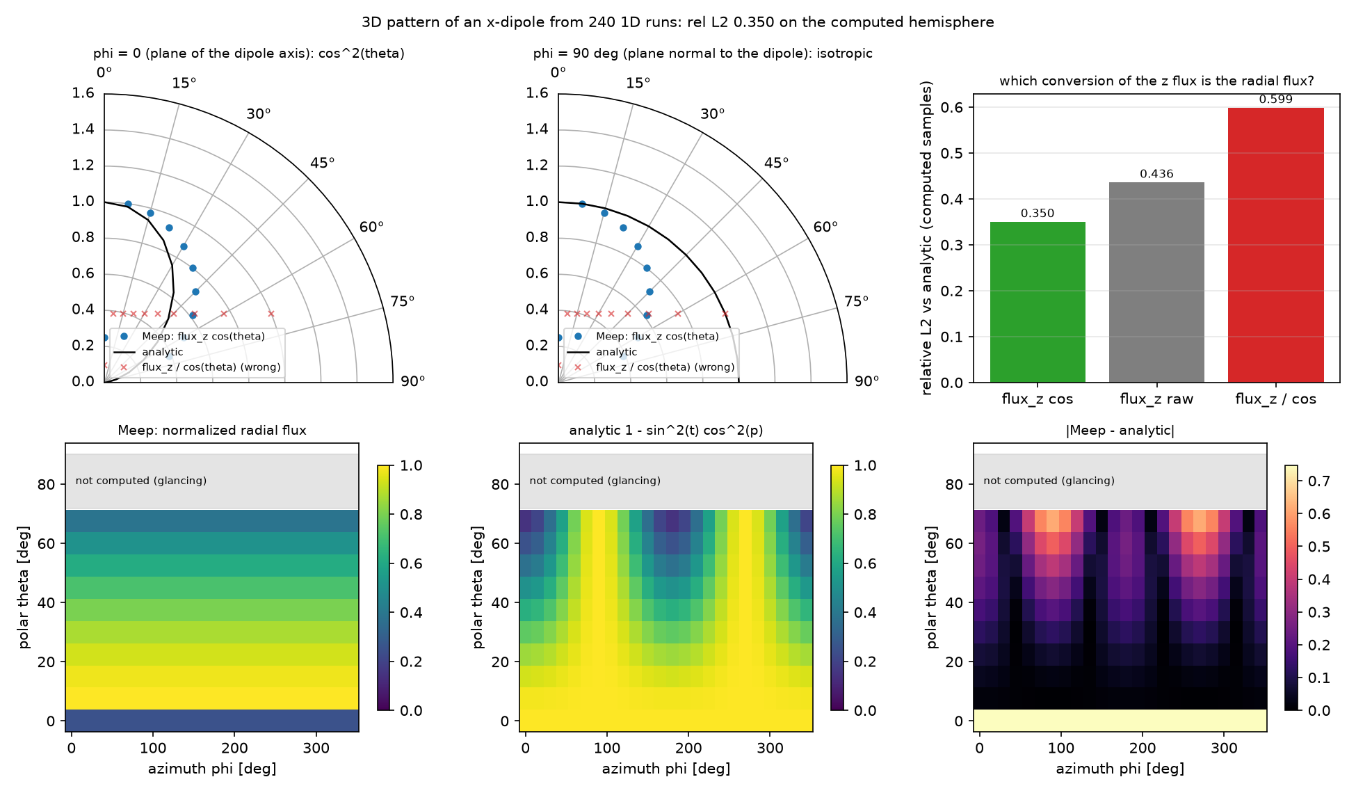
dimensions=1을 명시하고 k_point에 z 성분이 없었다. Meep 지도(왼쪽 아래)가 $\phi$에 전혀 의존하지 않고 $\theta=0$ 행만 어둡다. 두 증상이 각각 “횡방향 k가 무시됨”과 “k = 0이라 실수 field”의 지문이다. L2 0.35. 그림은 틀렸지만 어디가 틀렸는지를 말해 주기 때문에 남겨 둔다.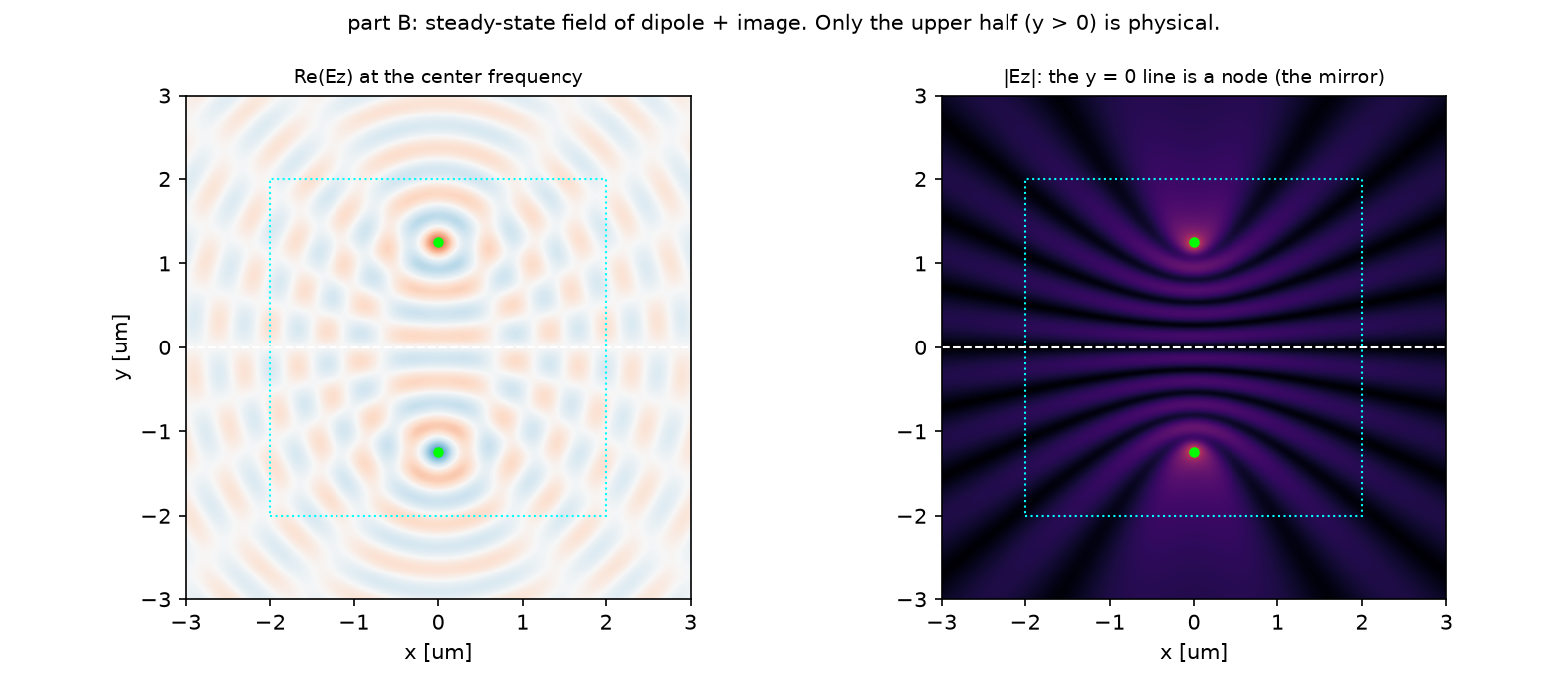
| 방법 | 비교 대상 | 상대 L2 |
|---|---|---|
| B: 2D near2far (Ez) | $\sin^2(kh\cos\theta)$, 50각 | 0.66% (peak bin 차이 0) |
| C: 1D Bloch (Ex, $\phi=90°$), 72° 아래 | $\sin^2(kh\cos\theta)$ | 6.8% |
| C: 같은 것, 85°까지 포함 | 〃 | 10.5% (상관 0.981) |
| C: 1D Bloch ($\phi=0$), 72° 아래 | $\cos^2\theta\,\sin^2(kh\cos\theta)$ | 6.0% |
| B vs C, 72° 아래 | 서로 | 6.4% |
예측과 비교
| 물리량 | 내 예측 (§2) | 시뮬레이션 | 판정 |
|---|---|---|---|
| 1D run 묶음 vs 해석 패턴 | 2% 안 | 0.22% | ✅ |
| 환산 인자 | $\cos\theta$ 곱 | 곱 0.22%, 나눔 76% | ✅ |
| $\phi=90°$ 단면 | 상수 | 상수 | ✅ |
| 2D PEC vs array factor | 1% 안 | 0.66% | ✅ |
| $y=0$의 $\lvert E_z\rvert$ | 0 | 최대의 0.012배 | ✅ |
| lobe 수 | 5개 | 5개, 최대 12.9° | ✅ |
| 1D Bloch PEC vs 2D | 2% 안 | 6.4% | ❌ (6.4%) |
| 72° 위의 1D run | 틀어짐 | 85°까지 넣으면 L2 10.5% | ✅ |
예측 여덟 중 일곱이 맞았고 하나가 틀렸다. 1D Bloch 방법은 거울 위에서도 lobe의 위치와 수를 정확히 재현하지만 진폭이 72° 아래에서도 6% 어긋난다. 원인은 두 가지로 본다. 거울 면이 Yee 격자의 반 칸(10 nm) 안에서 불확실해 $kh$가 0.12 rad 흔들리면 $\theta=0$의 lobe 진폭이 5% 바뀐다. 그리고 5° 간격 표본은 폭이 10° 남짓한 lobe의 봉우리와 골을 비껴 지나므로 정규화의 기준이 되는 최대값 자체가 표본 위치에 좌우된다. 2D near2far는 이 두 문제가 없고 0.66%다. 10_sources의 1D Bloch PEC 노트가 상관 0.947에서 멈춘 것은 같은 한계이고, 이 글은 glancing 각을 빼면 0.98, 넣으면 0.105의 L2로 그 경계를 숫자로 남긴다. 진공에서는 거울이 없으니 격자 반 칸 문제가 없고 0.22%가 나온다.
수렴성
| 변수 | 값 | 결과 | 비고 |
|---|---|---|---|
| A 각도 격자 | 13 × 24 (이 글) vs 30 × 50 (노트 0724) | L2 0.22% vs 0.22% | 표본 수는 L2를 바꾸지 않는다. 각 표본이 독립된 run이라 격자는 해상도가 아니라 그림의 촘촘함이다. 노트 0722의 1.99%는 고정 시간 종료의 값 |
| C glancing 포함 여부 | 72° 아래 / 85°까지 | 6.8% / 10.5% | 노트 0722의 상관 0.947은 glancing을 포함한 값이었다 |
| B 해상도 | 100 (이 글, 노트와 동일) | 0.66% | 노트 0.47%. 해상도 사다리는 직접 해보기 |
주장할 수 있는 것 / 없는 것
- 할 수 있는 것: x 쌍극자의 3D 패턴은 72° 아래에서 1D run 묶음으로 0.22% 안에 재현된다. $S_z\cos\theta$가 맞는 환산이다. 거울 위 쌍극자의 패턴은 image 이론의 array factor와 0.66% 안에서 같고, 1D 방법도 72° 아래에서는 같은 답을 준다.
- 할 수 없는 것: 72° 위의 방사 세기. 1D 방법은 그 영역을 계산하지 못하고, 이 글의 2D near2far도 그 영역의 수렴성을 따로 보지 않았다. 절대 power와 directivity. 손실 있는 금속 거울. y 편광과 다른 해상도로의 일반화.
원본 §6 · 흔한 실수
| 증상 | 원인 | 고치는 법 |
|---|---|---|
| flux가 각도에 무관, 패턴 L2 35% | dimensions=1을 명시해 횡방향 k가 무시됨 |
dimensions를 빼고 cell_size=(0, 0, sz)로만 1D를 만든다 |
| $\theta=0$ run만 power가 1/4 | $\mathbf k=0$이라 실수 field로 전환 | k_point에 z 성분 $f\cos\theta$를 넣어 항상 복소 field |
| 1D run이 끝나지 않음 | 위 설정 오류, 또는 glancing 각의 PML 정체 | 설정을 고치고, glancing 각은 고정 until_after_sources |
| 패턴이 $\theta$ 큰 쪽에서 과대 | $S_z/\cos\theta$ 환산 | $S_z\cos\theta$ |
| 반구 L2가 30%대 | 계산하지 않은 glancing 표본을 0으로 포함 | 계산한 표본만 비교하고 빈칸은 빈칸으로 그린다 |
| $y=0$이 antinode | image 부호 또는 phase=-1 누락 |
Ez는 odd, Hz는 even |
| lobe 각도가 전부 어긋남 | $k$에 배경 굴절률 누락 | $k=2\pi n/\lambda$, 파트 C의 k_point에도 n |
| near2far 패턴이 뒤틀림 | box 조각의 weight 부호 |
아래·왼쪽 조각 −1 |
| 파트 C에서 거울이 사라짐(L2 43%) | k_point가 셀 벽을 Bloch 주기로 바꿈 |
거울은 mp.metal 블록으로 geometry에 넣는다 |
| 1D Bloch의 lobe 진폭이 5% 어긋남 | 거울 면이 Yee 격자 반 칸(10 nm) 안에서 불확실, $kh$가 0.12 rad 흔들림 | 해상도를 올리거나 h를 격자에 맞춘다 |
원본 §7 · 직접 해보기
| 바꿀 것 | 예상 변화 | 확인할 수치 |
|---|---|---|
| 파트 A를 y 쌍극자로 | 패턴이 $\phi$ 방향으로 90° 돈다 | $\phi=0$ 단면이 상수가 되는지 |
GLANCING 0.95 → 0.99 |
72~82° 표본이 생기지만 오차가 큼 | 그 행의 |Meep − 해석| |
| 파트 B의 h를 0.3 µm로 | $kh=3.5$, lobe 1~2개 | peak 각도 |
| 파트 B 해상도 50 / 100 / 150 | L2 사다리 | 0.66%가 어디서 정체하는지 |
| 파트 B를 Hz 편광으로 | image 부호 +1, Mirror(Y, phase=+1) |
$y=0$이 antinode인지 |
code/dipole_pattern_3d.py 전체 (클릭하여 펼치기)
"""Meep Example 10 - 3D radiation pattern of a point dipole: a family of 1D Bloch runs, and a PEC mirror.

Post 01 showed a 2D point source radiating equally in all directions. This post asks the 3D question in two ways.
  A. Vacuum Ex dipole, 3D pattern WITHOUT a 3D cell: one 1D simulation per direction (theta, phi), each with a
     transverse Bloch wavevector k = f (sin t cos p, sin t sin p, 0). The z flux of each run, times cos(theta),
     is one angular sample of the 3D pattern. Compared with the analytic dipole pattern 1 - sin^2(t) cos^2(p).
  B. A dipole 1.25 um above a perfect-electric-conductor (PEC) mirror, 2D (Ez): the mirror is replaced by an
     opposite-sign image dipole plus an odd mirror symmetry, and the far field comes from a closed near2far box.
     Compared with the two-element array factor sin^2(k h cos t).
  C. The same mirror problem with the 1D Bloch method of part A (3D Ex dipole, PEC = metallic cell boundary):
     the two methods agree on the pattern away from grazing angles; near grazing the 1D method breaks down.

Run:  python dipole_pattern_3d.py     (~3 min on one core)
Out:  00_source.png, 01_layout.png, 02_layout_1d.png, 03_vacuum_pattern.png, 04_pec_field.png, 05_pec_pattern.png,
      06_anim_pec.gif, 07_anim_1d.gif, result.json   (-> ../assets/10/)
"""
import json
import os
import sys
import time

import numpy as np
import matplotlib
matplotlib.use("Agg")
import matplotlib.pyplot as plt
from matplotlib import animation
import meep as mp

sys.path.insert(0, os.path.dirname(os.path.abspath(__file__)))
from blogfig import Label, _badge, animate_fields, annotated_layout, record_frames, source_figure   # noqa: E402

HERE = os.path.dirname(os.path.abspath(__file__))
OUT = os.path.join(HERE, "..", "assets", "10")
os.makedirs(OUT, exist_ok=True)
t_all = time.time()


def rel_l2(a, b):
    a, b = np.asarray(a, float), np.asarray(b, float)
    return float(np.linalg.norm(a - b) / np.linalg.norm(b))


# =================================================================== A. vacuum dipole via 1D Bloch runs
# ---------------------------------------------------------------- (1) parameters (official dipole_in_vacuum_1D.py, smaller grid)
WL_A = 1.0                               # wavelength [um]; the pattern is scale-free
FCEN_A = 1 / WL_A
FWIDTH_A = 0.1 * FCEN_A
RES_A = 50
DPML_A, DAIR_A = 1.0, 10.0
SZ_A = DPML_A + DAIR_A + DPML_A
Z_SRC_A = -0.5 * DAIR_A                  # dipole at the bottom of the air gap (official)
Z_MON_A = 0.5 * DAIR_A                   # flux point at the top of the air gap
GLANCING = 0.95                          # skip k_perp > 0.95 f: PML cannot absorb nearly-parallel waves (official rule)
POLAR = np.radians(np.arange(0.0, 90.1, 7.5))      # 13 polar angles (0 = +z)
AZIM = np.radians(np.arange(0.0, 360.0, 15.0))     # 24 azimuth angles


def bloch_k(theta, phi, fcen, n_index=1.0):
    """Full wavevector of the outgoing plane wave, |k| = n f. The z component keeps k != 0 at theta = 0,
    so every run uses complex fields (a k = 0 run would switch to real fields and change the power scale by 4)."""
    return mp.Vector3(n_index * fcen * np.sin(theta) * np.cos(phi), n_index * fcen * np.sin(theta) * np.sin(phi), n_index * fcen * np.cos(theta))


def flux_1d(theta, phi, *, fcen, fwidth, n_index=1.0, sz=SZ_A, z_src=Z_SRC_A, z_mon=Z_MON_A, pml=None, geometry=(), component=mp.Ex, until=None):
    """One 1D run: Bloch k from (theta, phi), source at z_src, Poynting z-flux at z_mon.
    NOTE: do not pass dimensions=1. The cell size (0, 0, sz) already makes the run 1D, and an explicit dimensions=1
    silently drops the transverse k (the flux then no longer depends on the angle)."""
    sim = mp.Simulation(cell_size=mp.Vector3(0, 0, sz), resolution=RES_A, k_point=bloch_k(theta, phi, fcen, n_index),
                        default_material=mp.Medium(index=n_index), geometry=list(geometry),
                        boundary_layers=pml if pml is not None else [mp.PML(thickness=DPML_A, direction=mp.Z)],
                        sources=[mp.Source(mp.GaussianSource(fcen, fwidth=fwidth), component=component, center=mp.Vector3(0, 0, z_src), size=mp.Vector3())])
    mon = sim.add_flux(fcen, 0, 1, mp.FluxRegion(center=mp.Vector3(0, 0, z_mon), size=mp.Vector3(), direction=mp.Z))
    sim.run(until_after_sources=until if until is not None else mp.stop_when_fields_decayed(25, component, mp.Vector3(0, 0, z_mon), 1e-6))
    f = float(mp.get_fluxes(mon)[0]); sim.reset_meep()
    return f


t_a = time.time()
flux_z = np.full((len(POLAR), len(AZIM)), np.nan)
for i, th in enumerate(POLAR):
    if np.sin(th) > GLANCING:
        continue
    for j, ph in enumerate(AZIM):
        flux_z[i, j] = flux_1d(th, ph, fcen=FCEN_A, fwidth=FWIDTH_A)
n_runs = int(np.sum(~np.isnan(flux_z)))
computed = ~np.isnan(flux_z)
cos_t = np.cos(POLAR)[:, None]
radial = flux_z * cos_t                                   # official: radial flux = (kz / f) * flux_z
TH, PH = np.meshgrid(POLAR, AZIM, indexing="ij")
analytic_A = 1 - np.sin(TH) ** 2 * np.cos(PH) ** 2        # |E|^2 of an x-polarized dipole, up to a constant


def norm(p, mask):
    return p / np.nanmax(np.where(mask, p, np.nan))


err_mul = rel_l2(norm(radial, computed)[computed], norm(analytic_A, computed)[computed])
err_div = rel_l2(norm(flux_z / cos_t, computed)[computed], norm(analytic_A, computed)[computed])
err_raw = rel_l2(norm(flux_z, computed)[computed], norm(analytic_A, computed)[computed])
j0 = 0; j90 = int(np.argmin(np.abs(AZIM - np.pi / 2)))
err_phi0 = rel_l2(norm(radial, computed)[computed[:, j0], j0], norm(analytic_A, computed)[computed[:, j0], j0])
print(f"A: {n_runs} 1D runs ({len(POLAR)}x{len(AZIM)} grid, {int(np.sum(~computed))} glancing samples skipped) in {time.time() - t_a:.0f} s; "
      f"rel L2 vs analytic (computed samples): flux_z*cos = {err_mul:.4f}, flux_z/cos = {err_div:.4f}, flux_z raw = {err_raw:.4f}; phi=0 cut {err_phi0:.4f}")

# schematic of the 1D cell (plot2D has nothing to draw in 1D)
fig, ax = plt.subplots(figsize=(8.6, 3.2))
ax.axhspan(-0.5, 0.5, xmin=0, xmax=DPML_A / SZ_A, color="green", alpha=0.25); ax.axhspan(-0.5, 0.5, xmin=1 - DPML_A / SZ_A, xmax=1, color="green", alpha=0.25)
ax.plot([Z_SRC_A, Z_SRC_A], [-0.4, 0.4], color="red", lw=3); ax.plot(Z_MON_A, 0, "s", color="blue", ms=9)
th_demo = np.radians(45)
ax.annotate("", xy=(Z_SRC_A + 2.2 * np.cos(th_demo), 0.45 * np.sin(th_demo)), xytext=(Z_SRC_A, 0), arrowprops=dict(arrowstyle="->", color="purple", lw=1.8))
ax.text(Z_SRC_A + 1.4, 0.36, "k = f (sin t cos p, sin t sin p, cos t)\nonly the z axis is simulated", color="purple", fontsize=8)
for xy, step, color, txt, txy in (((-0.5 * SZ_A + 0.3, 0.42), 1, "dimgray", f"wl={WL_A} um, res={RES_A}\n{len(POLAR)} polar x {len(AZIM)} azimuth runs", (-0.5 * SZ_A + 0.6, 0.30)),
                                   ((Z_SRC_A, -0.42), 3, "red", "Ex dipole (GaussianSource)", (Z_SRC_A + 0.25, -0.46)),
                                   ((-0.5 * SZ_A + 0.5 * DPML_A, 0), 4, "green", "PML (both ends)", (-0.5 * SZ_A + 0.1, -0.15)),
                                   ((Z_MON_A, 0.12), 5, "blue", "flux point: Poynting z-flux", (Z_MON_A - 2.6, 0.18)),
                                   ((Z_MON_A, -0.12), 6, "purple", "decay watch point", (Z_MON_A - 1.9, -0.3))):
    _badge(ax, xy, step, color); ax.text(*txy, txt, fontsize=8, color=color)
ax.set_xlim(-0.5 * SZ_A, 0.5 * SZ_A); ax.set_ylim(-0.5, 0.5); ax.set_yticks([]); ax.set_xlabel("z [um]")
ax.set_title("part A: one 1D cell per direction; the transverse Bloch wavevector k_point picks the direction (theta, phi)", fontsize=9)
fig.tight_layout(); fig.savefig(os.path.join(OUT, "02_layout_1d.png"), dpi=150); plt.close(fig)

# pattern figure: two polar cuts + hemisphere maps
fig = plt.figure(figsize=(13, 7.6))
gs = fig.add_gridspec(2, 3)
for col, (j, lab, an) in enumerate(((j0, "phi = 0 (plane of the dipole axis): cos^2(theta)", np.cos(POLAR) ** 2),
                                    (j90, "phi = 90 deg (plane normal to the dipole): isotropic", np.ones_like(POLAR)))):
    ax = fig.add_subplot(gs[0, col], projection="polar")
    m = computed[:, j]
    ax.plot(POLAR[m], norm(radial, computed)[m, j], "o", color="tab:blue", ms=4, label="Meep: flux_z cos(theta)")
    ax.plot(POLAR, an, "-", color="k", lw=1.2, label="analytic")
    ax.plot(POLAR[m], norm(flux_z / cos_t, computed)[m, j], "x", color="tab:red", ms=4, alpha=0.6, label="flux_z / cos(theta) (wrong)")
    ax.set_theta_zero_location("N"); ax.set_theta_direction(-1); ax.set_thetamin(0); ax.set_thetamax(90); ax.set_rlim(0, 1.6)
    ax.set_title(lab, fontsize=9); ax.legend(fontsize=7, loc="lower left")
ax = fig.add_subplot(gs[0, 2])
ax.bar(["flux_z cos", "flux_z raw", "flux_z / cos"], [err_mul, err_raw, err_div], color=["tab:green", "tab:gray", "tab:red"])
for k_, v in enumerate([err_mul, err_raw, err_div]):
    ax.text(k_, v + 0.01, f"{v:.3f}", ha="center", fontsize=8)
ax.set_ylabel("relative L2 vs analytic (computed samples)"); ax.set_title("which conversion of the z flux is the radial flux?", fontsize=9); ax.grid(axis="y", alpha=0.3)
Td, Pd = np.degrees(POLAR), np.degrees(AZIM)
for col, (data, ttl, cmap, vmax) in enumerate(((norm(radial, computed), "Meep: normalized radial flux", "viridis", 1.0),
                                                (norm(analytic_A, computed), "analytic 1 - sin^2(t) cos^2(p)", "viridis", 1.0),
                                                (np.abs(norm(radial, computed) - norm(analytic_A, computed)), "|Meep - analytic|", "magma", None))):
    ax = fig.add_subplot(gs[1, col])
    pc = ax.pcolormesh(Pd, Td, np.where(computed, data, np.nan), cmap=cmap, vmin=0, vmax=vmax, shading="nearest")
    ax.axhspan(np.degrees(np.arcsin(GLANCING)), 90, color="lightgray", alpha=0.6); ax.text(5, 80, "not computed (glancing)", fontsize=7)
    ax.set_xlabel("azimuth phi [deg]"); ax.set_ylabel("polar theta [deg]"); ax.set_title(ttl, fontsize=9); fig.colorbar(pc, ax=ax, shrink=0.85)
fig.suptitle(f"3D pattern of an x-dipole from {n_runs} 1D runs: rel L2 {err_mul:.3f} on the computed hemisphere", fontsize=10)
fig.tight_layout(); fig.savefig(os.path.join(OUT, "03_vacuum_pattern.png"), dpi=150); plt.close(fig)

# GIF of one oblique 1D run (theta = 45 deg): Re(Ex) along z vs time
th_g = np.radians(45)
sim_g = mp.Simulation(cell_size=mp.Vector3(0, 0, SZ_A), resolution=RES_A, k_point=bloch_k(th_g, 0.0, FCEN_A),
                      boundary_layers=[mp.PML(thickness=DPML_A, direction=mp.Z)],
                      sources=[mp.Source(mp.GaussianSource(FCEN_A, fwidth=0.4 * FCEN_A), component=mp.Ex, center=mp.Vector3(0, 0, Z_SRC_A), size=mp.Vector3())])
sim_g.init_sim()
t0g = 5 / (0.4 * FCEN_A)
frames_g, times_g = [], []
sim_g.run(until=t0g - 2 / (0.4 * FCEN_A))
for i in range(50):
    sim_g.run(until=0.3)
    frames_g.append(np.real(sim_g.get_array(center=mp.Vector3(), size=mp.Vector3(0, 0, SZ_A), component=mp.Ex)))
    times_g.append(sim_g.meep_time())
zs = np.linspace(-0.5 * SZ_A, 0.5 * SZ_A, len(frames_g[0]))
lim_g = max(np.max(np.abs(f)) for f in frames_g)
fig_g, ax_g = plt.subplots(figsize=(7.6, 2.9))
ln, = ax_g.plot(zs, frames_g[0], color="tab:blue"); ax_g.set_ylim(-lim_g, lim_g); ax_g.set_xlim(zs[0], zs[-1])
ax_g.axvspan(zs[0], zs[0] + DPML_A, color="green", alpha=0.2); ax_g.axvspan(zs[-1] - DPML_A, zs[-1], color="green", alpha=0.2)
ax_g.axvline(Z_SRC_A, color="red", lw=1.5, label="source"); ax_g.axvline(Z_MON_A, color="blue", lw=1.5, ls="--", label="flux point")
ax_g.set_xlabel("z [um]"); ax_g.set_ylabel("Re(Ex)"); ax_g.legend(fontsize=7, loc="upper right"); ttl_g = ax_g.set_title("", fontsize=9)
fig_g.tight_layout()


def _upd(i):
    ln.set_ydata(frames_g[i]); ttl_g.set_text(f"one 1D run (theta = 45 deg): the pulse moves along z at c cos(theta)   t = {times_g[i]:.1f} um/c")
    return ln, ttl_g


animation.FuncAnimation(fig_g, _upd, frames=len(frames_g), blit=False).save(os.path.join(OUT, "07_anim_1d.gif"), writer=animation.PillowWriter(fps=10), dpi=80)
plt.close(fig_g); sim_g.reset_meep()

# =================================================================== B. dipole above a PEC mirror, 2D near2far with an image dipole
# ---------------------------------------------------------------- (1) parameters (official antenna_pec_ground_plane.py)
WL_B = 0.65
FCEN_B = 1 / WL_B
FWIDTH_B = 0.2 * FCEN_B
N_B = 1.2
H = 1.25                                 # dipole height above the mirror
RES_B = 100
DPML_B, DBULK = 0.5, 6.0
S_B = DBULK + 2 * DPML_B                 # 7 x 7 cell
R_FF = 1000 * WL_B
NANG = 50
THETA_B = np.linspace(0, 0.5 * np.pi, NANG)          # angle from the mirror normal (+y)
K_B = 2 * np.pi * N_B / WL_B
array_factor = np.sin(K_B * H * np.cos(THETA_B)) ** 2
array_factor /= array_factor.max()

sources_B = [mp.Source(mp.GaussianSource(FCEN_B, fwidth=FWIDTH_B), component=mp.Ez, center=mp.Vector3(0, H)),
             mp.Source(mp.GaussianSource(FCEN_B, fwidth=FWIDTH_B), component=mp.Ez, center=mp.Vector3(0, -H), amplitude=-1.0)]   # image dipole
symB = [mp.Mirror(mp.X), mp.Mirror(mp.Y, phase=-1)]                                                                        # odd in y -> Ez = 0 on y = 0 (PEC)
common_B = dict(cell_size=mp.Vector3(S_B, S_B), resolution=RES_B, boundary_layers=[mp.PML(DPML_B)], default_material=mp.Medium(index=N_B))
sim_B = mp.Simulation(sources=sources_B, symmetries=symB, **common_B)
BOX = 2.0                                                                                                                  # half-size of the near2far box (encloses both dipoles)
n2f = sim_B.add_near2far(FCEN_B, 0, 1,
                        mp.Near2FarRegion(center=mp.Vector3(0, BOX), size=mp.Vector3(2 * BOX, 0)),
                        mp.Near2FarRegion(center=mp.Vector3(0, -BOX), size=mp.Vector3(2 * BOX, 0), weight=-1),
                        mp.Near2FarRegion(center=mp.Vector3(BOX, 0), size=mp.Vector3(0, 2 * BOX)),
                        mp.Near2FarRegion(center=mp.Vector3(-BOX, 0), size=mp.Vector3(0, 2 * BOX), weight=-1))
dft_B = sim_B.add_dft_fields([mp.Ez], FCEN_B, 0, 1, center=mp.Vector3(), size=mp.Vector3(DBULK, DBULK))
annotated_layout(
    sim_B, os.path.join(OUT, "01_layout.png"), dpml=DPML_B, figsize=(6.6, 6.2), axis_step=1.0,
    title="part B: dipole above a PEC mirror = dipole + opposite image, odd mirror symmetry in y",
    params_text=f"wl={WL_B} um, n={N_B}\nh={H} um, res={RES_B}\nk h = {K_B * H:.1f}",
    params_xy=(-3.4, 3.1), pml_xy=(-3.0, -3.25), decay_point=None,
    labels=[Label("physical Ez dipole at y = +h", (0.05, H), (0.6, 2.4), step=3, color="red"),
            Label("image dipole at y = -h, amplitude -1", (0.05, -H), (0.6, -2.4), step=3, color="red"),
            Label("y = 0: Ez = 0 here (effective PEC)", (-1.2, 0.0), (-3.4, -0.9), step=2, color="black"),
            Label("closed near2far box (4 segments)", (BOX, 1.0), (0.4, 1.4), step=5, color="blue")])
source_figure(FCEN_B, FWIDTH_B, os.path.join(OUT, "00_source.png"), wl_scale=1000.0, wl_unit="nm", time_unit="um/c")
t_b = time.time()
sim_B.run(until_after_sources=mp.stop_when_dft_decayed(tol=1e-6))
ez_B = sim_B.get_dft_array(dft_B, mp.Ez, 0)
pattern_B = np.zeros(NANG)
for i, th in enumerate(THETA_B):
    ff = sim_B.get_farfield(n2f, mp.Vector3(R_FF * np.sin(th), R_FF * np.cos(th)))
    E = np.array(ff[:3]); Hf = np.array(ff[3:])
    S = np.real(np.cross(E, np.conj(Hf)))
    pattern_B[i] = np.hypot(S[0], S[1])
sim_B.reset_meep()
pattern_B /= pattern_B.max()
err_B = rel_l2(pattern_B, array_factor)
peak_B, peak_an = int(np.argmax(pattern_B)), int(np.argmax(array_factor))
node = float(np.max(np.abs(ez_B[:, ez_B.shape[1] // 2])) / np.max(np.abs(ez_B)))
print(f"B: 2D near2far pattern vs sin^2(k h cos theta): rel L2 {err_B:.4f}, peak bin Meep {peak_B} vs analytic {peak_an} "
      f"({np.degrees(THETA_B[peak_B]):.1f} deg), |Ez| on the y = 0 line / max = {node:.1e}; {time.time() - t_b:.0f} s")

ext_B = [-0.5 * DBULK, 0.5 * DBULK, -0.5 * DBULK, 0.5 * DBULK]
fig, ax = plt.subplots(1, 2, figsize=(10.5, 4.6))
lim = float(np.max(np.abs(ez_B)))
ax[0].imshow(np.real(ez_B).T, extent=ext_B, origin="lower", cmap="RdBu", vmin=-lim, vmax=lim, aspect="equal"); ax[0].set_title("Re(Ez) at the center frequency", fontsize=9)
ax[1].imshow(np.abs(ez_B).T, extent=ext_B, origin="lower", cmap="inferno", aspect="equal"); ax[1].set_title("|Ez|: the y = 0 line is a node (the mirror)", fontsize=9)
for a in ax:
    a.axhline(0, color="w", ls="--", lw=1.0); a.plot([0, 0], [H, -H], "o", color="lime", ms=4)
    a.add_patch(plt.Rectangle((-BOX, -BOX), 2 * BOX, 2 * BOX, fill=False, color="cyan", lw=1.0, ls=":")); a.set_xlabel("x [um]")
ax[0].set_ylabel("y [um]")
fig.suptitle("part B: steady-state field of dipole + image. Only the upper half (y > 0) is physical.", fontsize=10)
fig.tight_layout(); fig.savefig(os.path.join(OUT, "04_pec_field.png"), dpi=150); plt.close(fig)

# GIF: monitor-free run with a short pulse, both dipoles visible, node line marked
sim_gB = mp.Simulation(sources=[mp.Source(mp.GaussianSource(FCEN_B, fwidth=0.5 * FCEN_B), component=mp.Ez, center=mp.Vector3(0, H)),
                                mp.Source(mp.GaussianSource(FCEN_B, fwidth=0.5 * FCEN_B), component=mp.Ez, center=mp.Vector3(0, -H), amplitude=-1.0)],
                       symmetries=symB, **dict(common_B, resolution=50))
sim_gB.init_sim()
vol_gB = mp.Volume(center=mp.Vector3(), size=mp.Vector3(DBULK, DBULK))
t0B = 5 / (0.5 * FCEN_B)
frames_B, times_B = record_frames(sim_gB, vol_gB, mp.Ez, t_start=t0B - 2 / (0.5 * FCEN_B), t_end=t0B + 1.1 * 0.5 * DBULK * N_B * 1.5, n_frames=60)
animate_fields(frames_B, times_B, ext_B, os.path.join(OUT, "06_anim_pec.gif"), figsize=(5.6, 5.0), dpi=70,
               lines=[((-0.5 * DBULK, 0), (0.5 * DBULK, 0), "k", "mirror plane y = 0 (Ez node)"), ((-BOX, BOX), (BOX, BOX), "blue", "near2far box (top)")],
               points=[(0, H, "red", "dipole"), (0, -H, "orange", "image dipole (-1)")], title="dipole + image", legend_loc="lower right")
sim_gB.reset_meep()

# =================================================================== C. the mirror problem with the 1D Bloch method (3D Ex dipole above PEC)
# A k_point makes EVERY cell boundary Bloch-periodic, so the mirror cannot be the cell wall: it is a block of mp.metal
# (perfect electric conductor) at the bottom of the 1D cell. PML only at the top; background n = 1.2.
DMETAL = 0.5
SZ_C = DMETAL + H + DAIR_A + DPML_A
Z_BOT = -0.5 * SZ_C
Z_PEC = Z_BOT + DMETAL                               # mirror surface
Z_SRC_C = Z_PEC + H
Z_MON_C = Z_PEC + H + DAIR_A
mirror = [mp.Block(center=mp.Vector3(0, 0, Z_BOT + 0.5 * DMETAL), size=mp.Vector3(mp.inf, mp.inf, DMETAL), material=mp.metal)]
POLAR_C = np.radians(np.arange(0.0, 90.0, 5.0))      # includes grazing angles on purpose
T_C = 150.0                                          # fixed duration: at 85 deg the wave needs ~140 time units to cross 10 um of n = 1.2
flux_C = {}
for phi_deg in (90.0, 0.0):
    vals = [flux_1d(th, np.radians(phi_deg), fcen=FCEN_B, fwidth=0.1 * FCEN_B, n_index=N_B, sz=SZ_C, z_src=Z_SRC_C, z_mon=Z_MON_C,
                    pml=[mp.PML(thickness=DPML_A, direction=mp.Z, side=mp.High)], geometry=mirror, until=T_C) for th in POLAR_C]
    flux_C[phi_deg] = np.array(vals) * np.cos(POLAR_C)
af_C = np.sin(K_B * H * np.cos(POLAR_C)) ** 2
an_C = {90.0: af_C, 0.0: af_C * np.cos(POLAR_C) ** 2}             # phi=0: times the dipole's own cos^2
ok_C = np.sin(POLAR_C) <= GLANCING
res_C = {}
for phi_deg in (90.0, 0.0):
    p = flux_C[phi_deg] / flux_C[phi_deg][ok_C].max(); a = an_C[phi_deg] / an_C[phi_deg][ok_C].max()
    res_C[phi_deg] = {"pattern": p, "analytic": a, "err_in": rel_l2(p[ok_C], a[ok_C]), "err_all": rel_l2(p, a),
                      "corr_all": float(np.corrcoef(p, a)[0, 1])}
    print(f"C [phi = {phi_deg:.0f} deg]: 1D Bloch, {len(POLAR_C)} angles: rel L2 {res_C[phi_deg]['err_in']:.4f} below the glancing limit, "
          f"{res_C[phi_deg]['err_all']:.4f} with grazing angles included (correlation {res_C[phi_deg]['corr_all']:.4f})")
pB_on_C = np.interp(POLAR_C, THETA_B, pattern_B)
err_BC = rel_l2(res_C[90.0]["pattern"][ok_C], pB_on_C[ok_C])
print(f"B vs C: 2D near2far (Ez) vs 1D Bloch (Ex, phi = 90 deg) on the same angles: rel L2 {err_BC:.4f}")

fig = plt.figure(figsize=(13, 4.6))
ax = fig.add_subplot(1, 3, 1, projection="polar")
ax.plot(THETA_B, pattern_B, "-", color="tab:blue", lw=1.6, label="B: 2D near2far (Ez dipole)")
ax.plot(THETA_B, array_factor, "--", color="k", lw=1.2, label="analytic sin^2(k h cos t)")
ax.plot(POLAR_C[ok_C], res_C[90.0]["pattern"][ok_C], "o", color="tab:green", ms=4, label="C: 1D Bloch (Ex, phi = 90)")
ax.plot(POLAR_C[~ok_C], res_C[90.0]["pattern"][~ok_C], "x", color="tab:red", ms=6, label="C: grazing angles")
ax.set_theta_zero_location("N"); ax.set_theta_direction(-1); ax.set_thetamin(0); ax.set_thetamax(90); ax.set_rlim(0, 1.3)
ax.set_title(f"dipole {H} um above a PEC, k h = {K_B * H:.1f}", fontsize=9); ax.legend(fontsize=6.5, loc="lower left")
ax = fig.add_subplot(1, 3, 2, projection="polar")
ax.plot(POLAR_C[ok_C], res_C[0.0]["pattern"][ok_C], "o", color="tab:green", ms=4, label="C: 1D Bloch, phi = 0")
ax.plot(POLAR_C[~ok_C], res_C[0.0]["pattern"][~ok_C], "x", color="tab:red", ms=6, label="grazing")
ax.plot(POLAR_C, res_C[0.0]["analytic"], "--", color="k", lw=1.2, label="analytic cos^2(t) sin^2(k h cos t)")
ax.set_theta_zero_location("N"); ax.set_theta_direction(-1); ax.set_thetamin(0); ax.set_thetamax(90); ax.set_rlim(0, 1.3)
ax.set_title("phi = 0: array factor times the dipole's cos^2", fontsize=9); ax.legend(fontsize=6.5, loc="lower left")
ax = fig.add_subplot(1, 3, 3)
for phi_deg, c in ((90.0, "tab:green"), (0.0, "tab:olive")):
    ax.plot(np.degrees(POLAR_C), np.abs(res_C[phi_deg]["pattern"] - res_C[phi_deg]["analytic"]), "o-", color=c, ms=4, label=f"1D Bloch, phi = {phi_deg:.0f}")
ax.plot(np.degrees(THETA_B), np.abs(pattern_B - array_factor), "-", color="tab:blue", lw=1.4, label="2D near2far")
ax.axvspan(np.degrees(np.arcsin(GLANCING)), 90, color="lightgray", alpha=0.6); ax.text(np.degrees(np.arcsin(GLANCING)) + 1, 0.02, "glancing:\nPML fails", fontsize=7)
ax.set_xlabel("theta from the mirror normal [deg]"); ax.set_ylabel("|pattern - analytic| (normalized)"); ax.set_yscale("log"); ax.set_ylim(1e-4, 2)
ax.grid(alpha=0.3); ax.legend(fontsize=7); ax.set_title("where each method fails", fontsize=9)
fig.suptitle(f"B: rel L2 {err_B:.4f} (near2far) | C: {res_C[90.0]['err_in']:.4f} below 72 deg, {res_C[90.0]['err_all']:.3f} with grazing angles", fontsize=10)
fig.tight_layout(rect=[0, 0, 1, 0.92]); fig.savefig(os.path.join(OUT, "05_pec_pattern.png"), dpi=150); plt.close(fig)

if mp.am_master():
    with open(os.path.join(OUT, "result.json"), "w") as f:
        json.dump({"A": {"wl": WL_A, "res": RES_A, "n_polar": len(POLAR), "n_azimuth": len(AZIM), "n_runs": n_runs, "n_skipped": int(np.sum(~computed)),
                         "glancing_limit_deg": float(np.degrees(np.arcsin(GLANCING))), "err_mul": err_mul, "err_div": err_div, "err_raw": err_raw, "err_phi0": err_phi0},
                   "B": {"wl": WL_B, "n": N_B, "h": H, "res": RES_B, "kh": K_B * H, "box": BOX, "err": err_B, "peak_bin": [peak_B, peak_an],
                         "peak_deg": float(np.degrees(THETA_B[peak_B])), "node_ratio": node,
                         "pattern": pattern_B.tolist(), "analytic": array_factor.tolist(), "theta_deg": np.degrees(THETA_B).tolist()},
                   "C": {str(int(k_)): {"err_in": v["err_in"], "err_all": v["err_all"], "corr_all": v["corr_all"], "pattern": v["pattern"].tolist()} for k_, v in res_C.items()},
                   "B_vs_C": err_BC, "theta_C_deg": np.degrees(POLAR_C).tolist(),
                   "wall_s_total": time.time() - t_all, "meep": mp.__version__}, f, indent=2)
print(f"total {time.time() - t_all:.0f} s")
원본 실행 기록과 재현 환경
§4의 발췌 코드와 달리 전체 코드에는 1D 셀 설계도 그리기, 반구 지도, GIF 두 개, result.json 기록이 들어 있다. 그림 helper blogfig.py는 시리즈 공통이며 같은 폴더(code/)에 있다. 전체 코드와 helper: https://github.com/jin-castle/meep-examples/blob/main/code.
실행 결과 (2026-10-23 실행):
A: 240 1D runs (13x24 grid, 72 glancing samples skipped) in 201 s; rel L2 vs analytic (computed samples): flux_z*cos = 0.0022, flux_z/cos = 0.7585, flux_z raw = 0.5290; phi=0 cut 0.0012
B: 2D near2far pattern vs sin^2(k h cos theta): rel L2 0.0066, peak bin Meep 7 vs analytic 7 (12.9 deg), |Ez| on the y = 0 line / max = 1.2e-02; 3 s
C [phi = 90 deg]: 1D Bloch, 18 angles: rel L2 0.0675 below the glancing limit, 0.1052 with grazing angles included (correlation 0.9809)
C [phi = 0 deg]: 1D Bloch, 18 angles: rel L2 0.0599 below the glancing limit, 0.0601 with grazing angles included (correlation 0.9965)
B vs C: 2D near2far (Ez) vs 1D Bloch (Ex, phi = 90 deg) on the same angles: rel L2 0.0637
total 258 s
재현 환경: meep 1.33.0 · Python 3.11 · conda install -c conda-forge pymeep · 실행 python dipole_pattern_3d.py (약 4.3 min, 단일 코어)