MEEP EXAMPLES 04
직선 도파로에서 빛이 전부 나올까?
정답을 아는 직선 도파로로 source와 monitor를 검증합니다. 구조가 가두는 모드와 실제로 넣고 재는 모드를 구분합니다.
이 글을 읽고 나면
- guided mode와 유효 굴절률 n_eff의 의미를 설명한다.
- EigenModeSource와 mode monitor로 같은 모드의 투과율을 구한다.
- T ≈ 1의 검산과 해상도 비교로 수치 잔차를 판단한다.
먼저 알면 좋은 것 굴절률과 전반사, 01편의 source·펄스 시각, 02편의 PML을 알면 시작할 수 있습니다.
English summary
- What: a 2D silicon strip waveguide (0.5 µm wide, SiO₂ cladding) with the fundamental TE mode injected at one end and measured at the other.
- Result: T = 1.0000, R = 8×10⁻⁶ at 1.55 µm. Everything that goes in comes out. The 0.5 µm strip guides three TE modes (n_eff = 3.15, 2.59, 1.45); only mode 1 is injected and measured.
- Takeaway: start with a problem whose answer you already know. If T ≠ 1 here, the measurement setup is wrong, not the device.
- Code: full script at the bottom, ~2.5 min on one core (the baseline run is 34 s; the rest is the convergence check).
1. 관찰 · 빛이 따라가는 길 보기
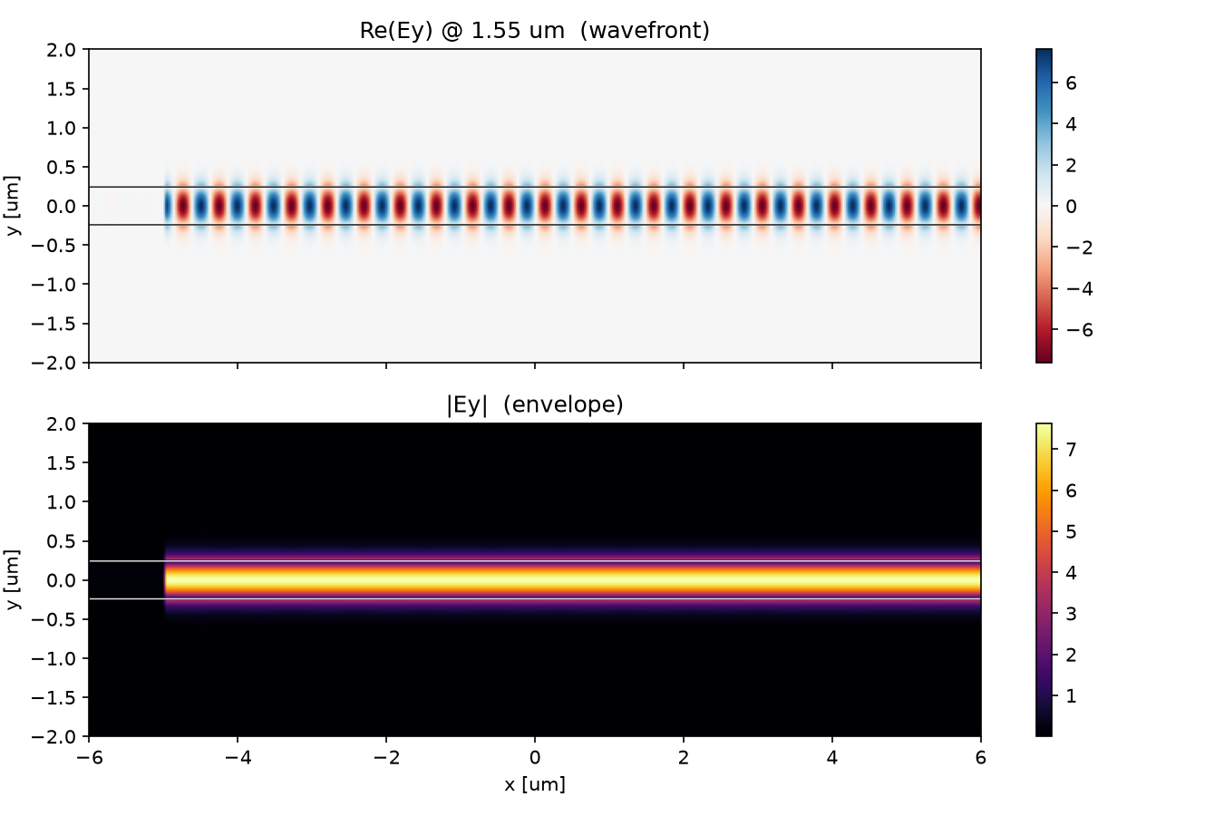
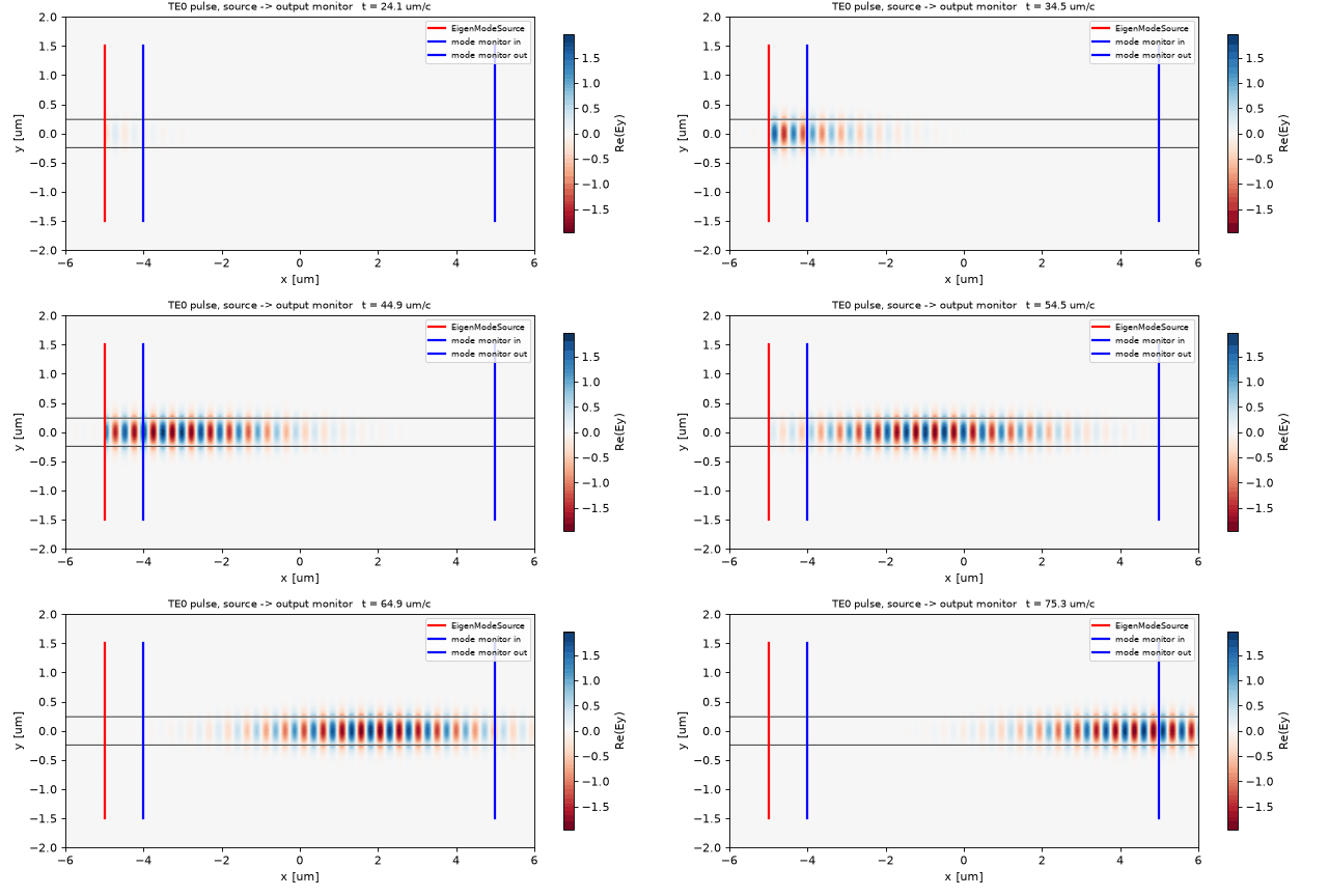
실리콘 띠에 기본 모드의 펄스를 넣습니다. 위 그림의 줄무늬가 띠를 따라 이어지고, 아래 포락선은 core 밖에서 약해집니다. 균일한 직선에는 빛을 꺾거나 되돌릴 불연속이 없습니다. 넣은 모드의 power가 반대쪽에서 그대로 나오는지 확인해 봅시다.
2. 예측 · 결과를 읽기 전에
기본 모드 투과율이 T ≈ 1이면, 이 도파로에 guided mode가 하나뿐이라는 뜻일까요?
예측의 근거 확인하기
두 번째입니다. source가 band 1만 넣고 monitor가 band 1에만 투영하면 mode 1 → mode 1의 T를 얻습니다. 구조가 지원하는 모드 수는 별도의 고유모드 계산으로 확인해야 합니다. 이 2D 단면은 세 모드를 가둡니다.
3. 원리 이해하기
모드는 단면이 허용하는 빛의 모양입니다
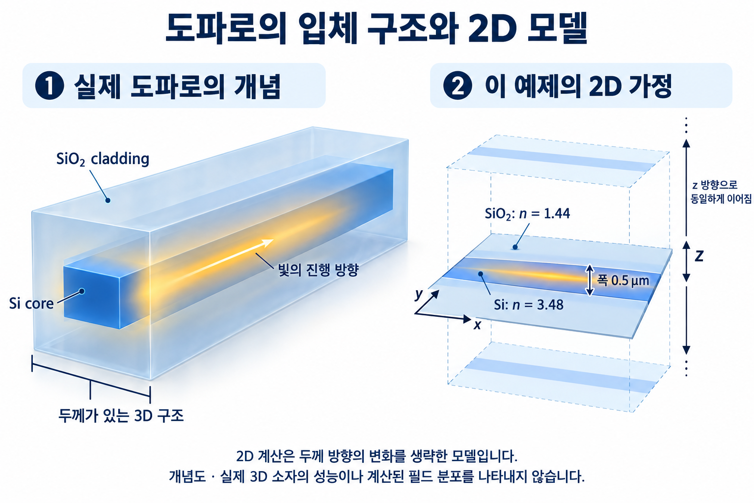
굴절률이 높은 Si core(n = 3.48)와 낮은 SiO₂ cladding(n = 1.44)의 경계가 빛을 가둡니다. 모드는 진행해도 횡방향 모양이 유지되는 장입니다. core 밖의 꼬리도 모드의 일부이므로 source와 monitor의 폭을 core보다 넓게 잡습니다.
유효 굴절률 n_eff = k/f는 진행 방향의 위상 변화율을 나타냅니다. 이 예제에서 1.44 < n_eff < 3.48이면 guided mode입니다. MPB 계산값은 band 1부터 3.153, 2.592, 1.447이며, 셋째는 cladding 굴절률 바로 위에 있습니다.
입력도 출력도 같은 모드를 기준으로 잽니다
EigenModeSource(eig_band=1)은 기본 모드 모양으로 주입합니다. get_eigenmode_coefficients(..., [1])은 입력과 출력의 장에서 같은 모드 성분을 골라냅니다. 앞으로 가는 입력 power로 앞으로 가는 출력 power를 나누면 T, 뒤로 돌아오는 입력면 power를 나누면 R입니다.
수식·기호와 원문의 예측 더 읽기
core(실리콘, n = 3.48)가 cladding(SiO₂, n = 1.44)보다 굴절률이 높으면 빛은 전반사로 core 안에 갇혀 전파한다. 갇힌 빛의 형태를 모드(mode)라 부르고, 가장 단순한 모양이 기본 모드 TE0이다. 균일한 직선에는 반사를 일으킬 불연속이 없으므로 손실 없이 전달된다.
\[T=\frac{\|a^{+}_{\mathrm{out}}\|^2}{\|a^{+}_{\mathrm{in}}\|^2},\qquad R=\frac{\|a^{-}_{\mathrm{in}}\|^2}{\|a^{+}_{\mathrm{in}}\|^2},\qquad T+R=1 \ (\text{lossless})\]| 기호 | 뜻 | 코드 변수 |
|---|---|---|
| $n_{\mathrm{core}}, n_{\mathrm{clad}}$ | core / cladding 굴절률 | n_si, n_sio2 |
| $a^{+}_{\mathrm{in}}$ | 입력 monitor에서 앞으로 가는 TE0 진폭 | ci.alpha[0, :, 0] |
| $a^{-}_{\mathrm{in}}$ | 입력 monitor에서 뒤로 가는(반사) TE0 진폭 | ci.alpha[0, :, 1] |
| $a^{+}_{\mathrm{out}}$ | 출력 monitor에서 앞으로 가는 TE0 진폭 | co.alpha[0, :, 0] |
가정과 유효 범위: 2D(z 방향 무한), lossless 재료. 폭 0.5 µm 슬랩은 TE 모드를 세 개 가두지만(아래 표) 기본 모드만 넣고 기본 모드에만 투영한다.
모드는 몇 개인가: n_eff 먼저
빛을 넣기 전에 이 단면이 어떤 모드를 가두는지 MPB로 푼다. Meep 안에서 sim.get_eigenmode를 부르면 같은 계산이 된다. 유효 굴절률 n_eff = k/f가 n_clad와 n_core 사이에 있으면 guided다.
sim.init_sim()
where = mp.Volume(center=mp.Vector3(src_x, 0), size=cross)   # the source cross-section
for band in (1, 2, 3):
    em = sim.get_eigenmode(fcen, mp.X, where, band, mp.Vector3(0.8 * n_si * fcen, 0, 0), parity=mp.ODD_Y)
    print(band, em.k.x / fcen)          # n_eff = k / f
| band | n_eff | guided? |
|---|---|---|
| 1 | 3.153 | 예 |
| 2 | 2.592 | 예 |
| 3 | 1.447 | 간신히 (n_clad = 1.44) |
EigenModeSource(eig_band=1)은 이 중 band 1만 넣고, get_eigenmode_coefficients(..., [1])은 band 1에만 투영한다. 그래서 이 글의 T는 “mode 1 → mode 1” 투과율이다.
결과 보기 전에 맞춰보기
| 물리량 | 내 예측 | 근거 |
|---|---|---|
| T | 1.000 (오차 10⁻³ 이내) | 반사·산란을 일으킬 것이 없다 |
| R | ≪ 10⁻³ | 불연속 없음. 격자 이산화 잔차만 남는다 |
| 필드 모양 | core 안에서 폭을 유지하며 전파, 밖에서 급감 | guided mode의 정의 |
| guided 모드 수 | 1개 | 폭 0.5 µm는 파장의 1/3이니 단일 모드일 것 |
판정 기준: |T − 1| > 0.01 또는 R > 10⁻³이면 구조가 아니라 source/monitor 배치나 정규화를 의심한다.
4. 실행 · 한 가지 조건만 바꾸기
먼저 원본을 실행해 기준 결과를 기록합니다. Meep 1.33.0 · Python 3.11, 기록된 단일 코어 실행 시간은 기준 약 34초, 수렴성 계산을 포함하면 약 2.5분입니다. 전체 코드와 공통 helper의 straight_waveguide.py와 blogfig.py를 같은 폴더에 두세요. 아래 전체 코드도 그대로 사용할 수 있습니다.
OMP_NUM_THREADS=1 python straight_waveguide.py
전체 코드의 w_core = 0.5를 w_core = 0.2로 바꾸고 다시 실행합니다. 다른 파라미터는 유지하세요. 출력의 n_eff by band에서 각 band를 cladding 굴절률 1.44와 비교해 guided mode 수를 다시 셉니다. 동시에 T가 기본 모드의 전달을 나타낸다는 점도 확인하세요. 폭이 줄어들면 구속이 약해질 것으로 예상하지만, 변경 후 n_eff와 모드 수는 직접 실행한 값으로 판정합니다.
배치에서 확인할 것
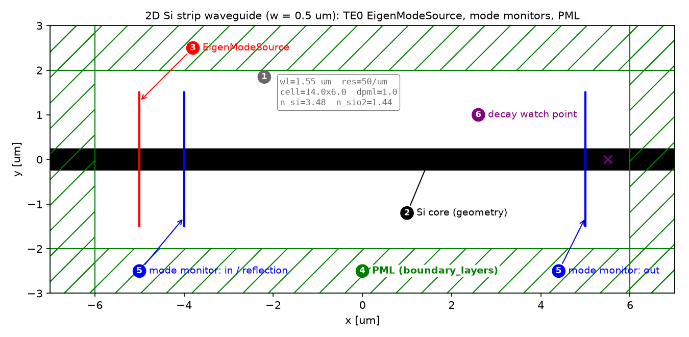
source는 x = −5, 입력 monitor는 −4, 출력 monitor는 +5입니다. core는 mp.inf로 PML까지 이어지고, source·monitor의 단면 폭은 3 µm로 모드 꼬리를 포함합니다.
설계도·파라미터와 source 파형
| 파라미터 | 값 | 왜 이 값인가 | 바꾸면 |
|---|---|---|---|
wl |
1.55 µm | 통신 표준 파장 | 모드 수·n_eff 변화 |
w_core |
0.5 µm | 기준 2D 단면, 기본 모드만 주입 | 넓히면 고차 모드 등장 |
resolution |
50 px/µm | core 25 px, 매질 내 파장 22 px | 20 이하: T가 1에서 벗어남 |
dpml |
1.0 µm | ≈ λ/1.5, 반사 억제 충분 | 얇으면 PML 반사로 R ↑ |
sx, sy |
14 × 6 µm | source·monitor·PML 사이 간격 확보 | 좁히면 monitor가 PML에 닿음 |
선 폭 cross |
3.0 µm | core + 바깥으로 새는 꼬리(evanescent tail) 포함 | core 폭만 잡으면 T < 1 |
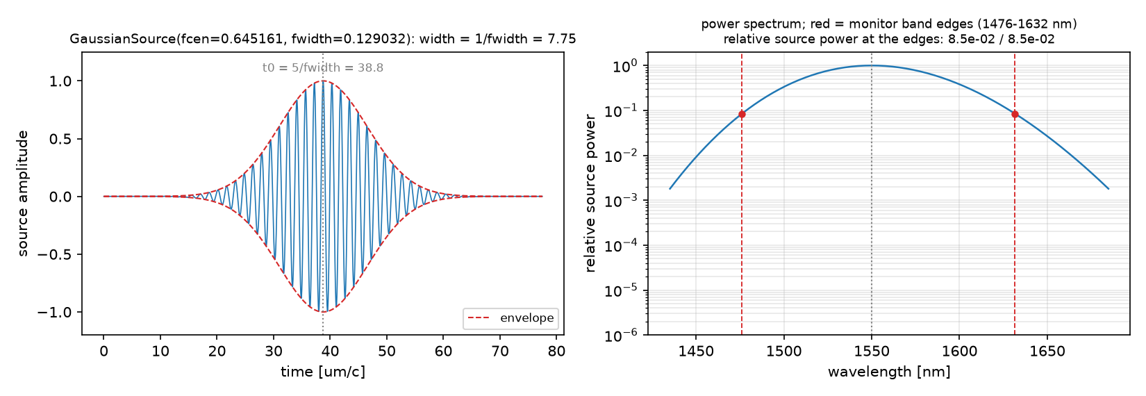
강의 노트북과의 차이: 강의 week 5는 n_core 3.4, 세로(+y) 도파로, MPB ModeSolver를 직접 부른다. 이 글은 공식 값 3.48, 가로 도파로, 같은 MPB를 sim.get_eigenmode로 Meep 안에서 부른다.
코드 따라가기 · 일곱 단계의 역할
읽는 순서: 단위·파라미터 → 재료·구조 → source → Simulation·경계 → monitor → 실행·종료 → 후처리. Meep 스크립트는 거의 항상 이 순서다.
① 단위와 파라미터 — 어떤 숫자를 고정하는가
import numpy as np
import meep as mp
import matplotlib.pyplot as plt

# Meep is unit-free. We choose 1 length unit = 1 um, so frequency = 1 / wavelength.
wl   = 1.55              # wavelength [um]
fcen = 1 / wl            # center frequency [1/um]
df   = 0.2 * fcen        # source bandwidth (Gaussian pulse)
nfreq = 11               # number of frequencies the monitors record

w_core = 0.5             # Si strip width [um]
n_si, n_sio2 = 3.48, 1.44

resolution = 50          # pixels per um  -> core = 25 px, lambda/n_si = 22 px
dpml = 1.0               # PML thickness [um]
sx, sy = 14.0, 6.0       # cell size [um], PML included
- 무엇: 길이 단위(µm)를 정하고, 그 단위로 파장·주파수·구조 치수·격자 밀도를 고정한다.
- 왜: Meep에는 단위가 없다. 1 = 1 µm로 정하면 주파수 단위는 1/µm이고, 파장 1.55 µm는 f = 0.645다.
- 틀리면:
resolution이 낮으면 core가 몇 픽셀로만 표현되어 모드 형태가 왜곡되고 T가 1에서 벗어난다.df가 너무 좁으면 펄스가 길어져 실행 시간이 늘어난다.
함정:
fcen = 1.55라고 쓰는 실수. Meep의 주파수는 파장의 역수다.
② 재료와 구조 — 무엇이 어디에 있는가
geometry = [mp.Block(center=mp.Vector3(0, 0),
                     size=mp.Vector3(mp.inf, w_core),   # infinite in x: runs straight through the PML
                     material=mp.Medium(index=n_si))]
# background (cladding) is set later via default_material=SiO2
- 무엇: 폭 0.5 µm, 길이 무한한 실리콘 띠 하나.
- 왜: 길이를
mp.inf로 두면 도파로가 PML 안까지 이어진다. PML은 경계를 가로질러 이어지는 구조를 흡수할 때 반사가 가장 적다. - 틀리면: cell보다 짧게 두면 끝면에서 반사가 생겨 R이 커진다.
③ Source — 빛을 어떻게 넣는가
cross = mp.Vector3(0, 3.0)   # a vertical line 3 um tall: wider than the core to include the evanescent tail

sources = [mp.EigenModeSource(src=mp.GaussianSource(fcen, fwidth=df),
                              center=mp.Vector3(-5.0, 0), size=cross,
                              eig_band=1,               # 1-indexed: the fundamental mode
                              eig_parity=mp.ODD_Y)]     # 2D TE polarization (Ey, Hx, Hz)
- 무엇: x = −5 위치의 세로선에서, 도파로의 기본 모드 모양으로 가우시안 펄스를 주입한다.
- 왜: 점 source나 평면파를 넣으면 모드에 맞지 않는 성분이 함께 들어가 반사·방사 잡음을 만든다.
EigenModeSource는 MPB로 모드를 먼저 풀어 그 모양대로 넣으므로 TE0만 들어간다. - 틀리면:
eig_parity를EVEN_Y로 두면 2D에서는 TM이 되어 전혀 다른 모드를 넣는다.size를 core 폭만큼만 잡으면 꼬리가 잘려 T < 1.
함정:
eig_band=0은 없다. 1부터 센다.
④ Simulation과 경계 — 계산 상자와 PML
sim = mp.Simulation(cell_size=mp.Vector3(sx, sy),
                    resolution=resolution,
                    boundary_layers=[mp.PML(dpml)],        # absorbing layer on all four sides
                    geometry=geometry,
                    sources=sources,
                    default_material=mp.Medium(index=n_sio2))

sim.plot2D()                       # ALWAYS look at the layout before running
plt.savefig("01_layout.png", dpi=150)
- 무엇: 지금까지 만든 재료·구조·source를 14 × 6 µm 상자에 넣고, 네 변에 1 µm PML을 두른다.
- 왜: PML(perfectly matched layer)은 상자 경계에 닿은 빛을 반사 없이 흡수해 무한히 넓은 공간을 흉내 낸다.
plot2D가 §3 그림을 만든다. 실행 전에 한 번 본다. - 틀리면:
boundary_layers를 빼면 경계가 거울이 되어 빛이 되돌아오고 R이 커진다.
⑤ Monitor — 무엇을 재는가
mon_in  = sim.add_mode_monitor(fcen, 0.1 * fcen, nfreq,
                               mp.ModeRegion(center=mp.Vector3(-4.0, 0), size=cross))
mon_out = sim.add_mode_monitor(fcen, 0.1 * fcen, nfreq,
                               mp.ModeRegion(center=mp.Vector3(+5.0, 0), size=cross))

# optional: steady-state field map of the whole non-PML region (for the figure in section 5)
dft = sim.add_dft_fields([mp.Ey], fcen, 0, 1,
                         where=mp.Volume(center=mp.Vector3(), size=mp.Vector3(sx - 2*dpml, sy - 2*dpml)))
- 무엇: source 바로 뒤(x = −4)와 반대쪽 끝(x = +5)에 모드 분해용 monitor 두 개, 그리고 전체 영역의 정상상태 필드 저장.
- 왜: 입력 monitor 하나로 앞으로 가는 양과 뒤로 오는 양(반사)을 동시에 분리할 수 있다. 그래서 반사 monitor를 source 앞이 아니라 뒤에 둔다.
- 틀리면: monitor를 source와 같은 x에 두면 주입 중인 필드와 섞여 계수가 오염된다. PML 안에 두면 흡수된 값을 잰다.
⑥ 실행과 종료 조건 — 언제 멈추는가
sim.run(until_after_sources=mp.stop_when_fields_decayed(
            25,                     # check every 25 time units
            mp.Ey,                  # which field component to watch
            mp.Vector3(5.5, 0),     # where to watch: just past the output monitor
            1e-6))                  # stop when |Ey|^2 has decayed to 1e-6 of its peak
- 무엇: source가 꺼진 뒤, 출력 monitor 근처의 필드가 최대값의 10⁻⁶으로 줄어들 때까지 돈다.
- 왜: 펄스가 monitor를 완전히 지나가야 주파수 분해(DFT)가 정확하다. 고정 시간(
until=200)은 구조가 바뀌면 틀릴 수 있어서 쓰지 않는다. - 틀리면: 너무 일찍 멈추면 monitor에 펄스 꼬리가 덜 들어와 T가 1보다 작게 나오고, 스펙트럼에 물결이 생긴다.
⑦ 후처리 — 숫자로 바꾸기
ci = sim.get_eigenmode_coefficients(mon_in,  [1], eig_parity=mp.ODD_Y)
co = sim.get_eigenmode_coefficients(mon_out, [1], eig_parity=mp.ODD_Y)

p_in_fwd  = np.abs(ci.alpha[0, :, 0])**2    # forward power at the input monitor   (a_in+)
p_in_back = np.abs(ci.alpha[0, :, 1])**2    # backward power at the input monitor  (a_in-)
p_out_fwd = np.abs(co.alpha[0, :, 0])**2    # forward power at the output monitor  (a_out+)

T = p_out_fwd / p_in_fwd                    # section 2, first formula
R = p_in_back / p_in_fwd                    # section 2, second formula
ic = nfreq // 2                             # index of the center frequency
print(f"T = {T[ic]:.4f}, R = {R[ic]:.2e}, T+R = {T[ic]+R[ic]:.4f}")
- 무엇: 두 monitor의 필드를 TE0 모드에 투영해 진폭 $a^{\pm}$를 얻고, 원문 예측의 식으로 T·R을 계산한다.
- 왜:
alpha[band, freq, direction]의 마지막 축이 0 = 앞, 1 = 뒤다. 입력 monitor의 뒤 성분이 곧 반사다. - 틀리면:
eig_parity를 source와 다르게 주면 다른 모드에 투영되어 T가 엉뚱하게 나온다.
5. 해석 · 숫자로 확인하고 한계 읽기
1.55 µm에서 T = 1.0000, R = 8.0 × 10⁻⁶입니다. 1.48–1.63 µm 대역에서도 T는 0.99999–1.00001입니다. 이것은 기본 모드 주입·측정·정규화가 직선 기준에서 일관되게 동작한다는 검산입니다.
전체 flux의 투과율도 1.0000이고, 입력 flux 중 mode 1의 몫은 0.9999입니다. 이 직선에서는 거의 같지만, 다른 구조에서 전체 flux와 특정 모드 power는 서로 다를 수 있습니다. 둘을 비교하거나 빼려면 분모부터 통일해야 합니다.
전체 결과·예측 비교·수렴성 표
| 물리량 | 값 | 비교 대상 |
|---|---|---|
| T @ 1.55 µm | 1.0000 | 이론 1 |
| R @ 1.55 µm | 8.0 × 10⁻⁶ | 이론 0 |
| T + R | 1.0000 | 에너지 보존 |
| T (1.48–1.63 µm) | 0.99999–1.00001 | 대역 전체에서 평탄 |
전체 flux와 modal power
add_mode_monitor는 flux monitor이기도 하다. 같은 단면에서 두 가지 수를 뽑을 수 있다.
| 양 | 분모 | 값 @ 1.55 µm |
|---|---|---|
| T (modal) = |a_out+|² / |a_in+|² | 입사 mode-1 power | 1.0000 |
| T_total = flux_out / flux_in | 입사면 전체 flux | 1.0000 |
| 입사 flux 중 mode 1의 몫 = |a_in+|² / flux_in | 입사면 전체 flux | 0.9999 |
직선에서는 셋이 같다. source가 넣은 power의 99.99%가 mode 1이고, 다른 모드로 새거나 방사되는 것이 없기 때문이다. 05편의 bend에서는 전체 flux와 mode-1 power가 갈라지고, 그 차이가 방사 손실이다. 분모가 다른 두 수를 서로 빼면 손실이 음수로 나오는 일이 생기므로, 손실을 계산할 때는 분모를 하나로 맞춘다.
수렴성
| resolution | dpml | T | R | 비고 |
|---|---|---|---|---|
| 50 | 1.0 | 1.000000 | 8.0 × 10⁻⁶ | 기준 |
| 25 | 1.0 | 0.999996 | 2.1 × 10⁻⁴ | 해상도 절반 |
| 70 | 1.0 | 1.000000 | 1.4 × 10⁻⁶ | 해상도 1.4배 |
| 50 | 0.5 | 1.000000 | 8.1 × 10⁻⁶ | PML 절반 |
T는 해상도 25에서도 1에 10⁻⁵ 안으로 붙는다. R은 해상도에 따라 10⁻⁴에서 10⁻⁶으로 내려가고 PML 두께에는 둔감하다. 이 구조에서 R은 PML 반사가 아니라 격자 이산화 잔차다.
예측과 비교
| 물리량 | 내 예측 (원문 예측) | 시뮬레이션 | 판정 |
|---|---|---|---|
| T | 1.000 ± 0.001 | 1.0000 | ✅ |
| R | ≪ 10⁻³ | 8 × 10⁻⁶ | ✅ |
| 필드 모양 | core 안에 갇힘 | 그림 확인 | ✅ |
| guided 모드 수 | 1개 | 3개 (n_eff 3.15, 2.59, 1.45) | ❌ |
T·R·필드는 예측대로다. 직선에는 반사원이 없으니 맞아야 하는 결과이고, 이 값은 source·monitor·PML·정규화 설정이 옳다는 증거로 쓴다.
모드 수는 틀렸다. 슬랩 도파로의 V수 $V = (\pi w/\lambda)\sqrt{n_{\mathrm{core}}^2 - n_{\mathrm{clad}}^2} = 3.2$는 π를 넘으므로 TE 모드가 세 개 갇히고, 셋째는 n_eff = 1.447로 cladding(1.44) 바로 위에 걸려 있다. 그런데도 T = 1이 나온 이유는 EigenModeSource가 band 1만 넣고 mode monitor가 band 1에만 투영하기 때문이다. 모드가 여럿인 도파로에서 투과율을 말할 때는 어느 모드의 투과율인지 같이 말해야 한다.
검증 체크: T + R = 1.0000 · source(x = −5)와 monitor(x = −4, +5) 모두 PML(|x| > 6) 밖 · 종료는 field decay 기준.
주장할 수 있는 것 / 없는 것
- 할 수 있는 것: 이 설정에서 mode 1 → mode 1 투과율은 1이고, 설정(source, monitor, PML, 정규화)은 신뢰할 수 있다.
- 할 수 없는 것: 3D SOI 도파로의 값. 2D 슬랩이라 유효 굴절률도 모드 수도 3D와 다르다. R의 둘째 자리 이하는 해상도에 따라 변한다.
6. 확인 · 내 말로 설명하기
1. 세 guided mode가 있는데도 T = 1이 나오는 이유는 무엇인가요?
답과 이유 확인하기
구조가 지원하는 모드와 실제로 여기된 모드는 다릅니다. source가 band 1을 넣고 monitor가 band 1에 투영하므로, 균일한 직선에서 같은 모드가 그대로 전달되는지를 잰 값입니다.
2. source와 monitor의 선 폭을 core 폭으로만 줄이면 무엇을 놓치나요?
답과 이유 확인하기
core 바깥의 evanescent tail도 모드의 일부입니다. source에서는 주입 모양을 자르고 monitor에서는 장의 일부를 빠뜨릴 수 있으므로, T 변화만으로 어느 한쪽만의 문제라고 단정할 수 없습니다.
7. 코드와 참고 자료
이 예제가 쓰이는 곳
직선 실리콘 도파로에 빛을 넣으면 반대쪽에서 전부 나와야 한다. 이 글은 그것을 Meep으로 확인한다. 답(T = 1)을 아는 문제를 먼저 고른 이유는, 빛을 넣는 source와 재는 monitor가 제대로 동작하는지를 구조와 분리해서 보기 위해서다. 여기서 1이 안 나오면 뒤에 어떤 구조를 돌려도 결과를 믿을 수 없다.
어디에 쓰이는가
직선 도파로는 실리콘 포토닉스의 배선이고, 그 위의 모든 부품은 이 글의 source와 monitor로 잰다.
| 응용 | 이 글의 어떤 것을 쓰는가 | 그 다음에 필요한 것 |
|---|---|---|
| 실리콘 포토닉스 배선(데이터센터 광연결, 트랜시버) | guided mode, n_eff, 단일 모드 조건 | 05편 bend, 29편 taper |
| 도파로 단면 설계(폭·두께 선택) | MPB n_eff 표, 세 모드의 존재 | 24편 밴드 구조 |
| 모든 도파로 부품의 투과율 측정 기준 | EigenModeSource + mode monitor, T = 1 교정 | 05·09편 |
| 광섬유–칩 결합기, 변조기, 광 스위치 | 입력 모드의 정의 | 30편 GDS 부품 |
흔한 실수와 해결 방법
| 증상 | 원인 | 고치는 법 |
|---|---|---|
| T ≈ 0.9 이하 | source/monitor 선 폭이 core만큼만 | cross를 core보다 넓게 (여기선 3 µm) |
| T가 들쭉날쭉한 스펙트럼 | 종료가 너무 빠름 | stop_when_fields_decayed 임계값 낮추기 |
| 전혀 다른 모드 모양 | 2D에서 EVEN_Y 사용 |
2D TE는 ODD_Y |
eig_band=0 오류 |
0-index로 착각 | 1부터 |
| R이 10⁻³ 이상 | PML 얇음 또는 구조가 PML 전에 끊김 | dpml ≥ λ/2, 길이 mp.inf |
원문의 추가 탐구 아이디어
| 바꿀 것 | 예상 변화 | 확인할 수치 |
|---|---|---|
resolution 50 → 20 |
T가 1에서 조금 벗어남 | |T − 1| |
w_core 0.5 → 0.2 µm |
band 2·3의 n_eff가 n_clad 아래로 내려가 단일 모드가 됨 | n_eff 표 |
dpml 1.0 → 0.2 µm |
PML 반사로 R 증가 | R |
straight_waveguide.py (클릭해서 펼치기)
"""Meep Example 04 - Straight waveguide and guided modes.

2D silicon strip waveguide in SiO2. Find the guided mode(s) and their effective index with
the eigenmode solver, inject the fundamental TE mode with EigenModeSource, and measure
modal transmission T and reflection R with mode monitors. Expected: T = 1, R = 0.
Then compare total flux with modal power, and check convergence in resolution and PML.

Run:  python straight_waveguide.py            (~3 min on one core: baseline + 2 convergence runs)
Out:  00_source.png, 01_layout.png, 02_field.png, 03_animation.gif, result.json  (-> ../assets/04/)
"""
import json
import os
import sys
import time

import numpy as np
import matplotlib
matplotlib.use("Agg")
import meep as mp

sys.path.insert(0, os.path.dirname(os.path.abspath(__file__)))
from blogfig import Label, animate_fields, annotated_layout, field_figure, record_frames, source_figure   # noqa: E402

OUT = os.path.join(os.path.dirname(os.path.abspath(__file__)), "..", "assets", "04")
os.makedirs(OUT, exist_ok=True)

# ---------------------------------------------------------------- (1) units & parameters
# Meep is unit-free. We choose 1 length unit = 1 um, so frequency = 1 / wavelength.
wl   = 1.55              # wavelength [um]
fcen = 1 / wl            # center frequency [1/um]
df   = 0.2 * fcen        # source bandwidth (Gaussian pulse)
df_mon = 0.1 * fcen      # monitor bandwidth
nfreq = 11               # number of frequencies the monitors record

w_core = 0.5             # Si strip width [um]
n_si, n_sio2 = 3.48, 1.44

RESOLUTION = 50          # pixels per um  -> core = 25 px, lambda/n_si = 22 px
DPML = 1.0               # PML thickness [um]
sx, sy = 14.0, 6.0       # cell size [um], PML included

# ---------------------------------------------------------------- (2) materials & geometry
geometry = [mp.Block(center=mp.Vector3(0, 0),
                     size=mp.Vector3(mp.inf, w_core),   # infinite in x: runs straight through the PML
                     material=mp.Medium(index=n_si))]
# background (cladding) is set below via default_material = SiO2

# ---------------------------------------------------------------- (3) source
cross = mp.Vector3(0, 3.0)   # a vertical line 3 um tall: wider than the core to include the evanescent tail
src_x, mon_in_x, mon_out_x = -5.0, -4.0, +5.0
PARITY = mp.ODD_Y            # 2D TE polarization (Ey, Hx, Hz)

sources = [mp.EigenModeSource(src=mp.GaussianSource(fcen, fwidth=df),
                              center=mp.Vector3(src_x, 0), size=cross,
                              eig_band=1,               # 1-indexed: the fundamental mode
                              eig_parity=PARITY)]
decay_pt = (mon_out_x + 0.5, 0)   # where stop_when_fields_decayed watches (step 6)


# ---------------------------------------------------------------- (4) simulation & boundaries
def build(resolution=RESOLUTION, dpml=DPML):
    """Simulation plus its two mode monitors. One function so every run is set up the same way."""
    sim = mp.Simulation(cell_size=mp.Vector3(sx, sy),
                        resolution=resolution,
                        boundary_layers=[mp.PML(dpml)],        # absorbing layer on all four sides
                        geometry=geometry,
                        sources=sources,
                        default_material=mp.Medium(index=n_sio2))
    # ------------------------------------------------------------ (5) monitors
    mon_in = sim.add_mode_monitor(fcen, df_mon, nfreq,
                                  mp.ModeRegion(center=mp.Vector3(mon_in_x, 0), size=cross))
    mon_out = sim.add_mode_monitor(fcen, df_mon, nfreq,
                                   mp.ModeRegion(center=mp.Vector3(mon_out_x, 0), size=cross))
    return sim, mon_in, mon_out


def run_and_measure(sim, mon_in, mon_out):
    # ------------------------------------------------------------ (6) run & stop condition
    sim.run(until_after_sources=mp.stop_when_fields_decayed(
                25,                         # check every 25 time units
                mp.Ey,                      # which field component to watch
                mp.Vector3(*decay_pt),      # where to watch: just past the output monitor
                1e-6))                      # stop when |Ey|^2 has decayed to 1e-6 of its peak
    # ------------------------------------------------------------ (7) post-processing
    ci = sim.get_eigenmode_coefficients(mon_in,  [1], eig_parity=PARITY)
    co = sim.get_eigenmode_coefficients(mon_out, [1], eig_parity=PARITY)
    p_in_fwd  = np.abs(ci.alpha[0, :, 0]) ** 2    # forward mode-1 power at the input monitor   (a_in+)
    p_in_back = np.abs(ci.alpha[0, :, 1]) ** 2    # backward mode-1 power at the input monitor  (a_in-)
    p_out_fwd = np.abs(co.alpha[0, :, 0]) ** 2    # forward mode-1 power at the output monitor  (a_out+)
    flux_in  = np.array(mp.get_fluxes(mon_in))    # TOTAL power through the input plane (all modes, net)
    flux_out = np.array(mp.get_fluxes(mon_out))   # TOTAL power through the output plane
    return {
        "T": p_out_fwd / p_in_fwd,                # modal transmission  (section 2, first formula)
        "R": p_in_back / p_in_fwd,                # modal reflection    (section 2, second formula)
        "T_total": flux_out / flux_in,            # total-flux transmission
        "mode1_fraction_in": p_in_fwd / flux_in,  # how much of the injected power is really mode 1
        "freqs": np.array(mp.get_flux_freqs(mon_in)),
    }


t_all = time.time()
ic = nfreq // 2

# ================================================================ baseline run with figures
sim, mon_in, mon_out = build()

# source waveform and spectrum (same GaussianSource the EigenModeSource wraps)
src_info = source_figure(fcen, df, os.path.join(OUT, "00_source.png"), mon_fcen=fcen, mon_df=df_mon,
                         wl_scale=1000.0, wl_unit="nm", time_unit="um/c")

annotated_layout(
    sim, os.path.join(OUT, "01_layout.png"), dpml=DPML,
    title="2D Si strip waveguide (w = 0.5 um): TE0 EigenModeSource, mode monitors, PML",
    params_text=f"wl={wl} um  res={RESOLUTION}/um\ncell={sx}x{sy}  dpml={DPML}\nn_si={n_si}  n_sio2={n_sio2}",
    params_xy=(-2.2, 1.85), decay_point=decay_pt, decay_text_xy=(2.6, 1.0),
    labels=[
        Label("Si core (geometry)", (1.5, 0.0), (1.0, -1.2), step=2, color="black"),
        Label("EigenModeSource", (src_x, 1.3), (src_x + 1.2, 2.5), step=3, color="red"),
        Label("mode monitor: in / reflection", (mon_in_x, -1.3), (mon_in_x - 1.0, -2.5), step=5, color="blue"),
        Label("mode monitor: out", (mon_out_x, -1.3), (mon_out_x - 0.6, -2.5), step=5, color="blue"),
    ])

# guided modes of the cross-section: effective index n_eff = k / f  (MPB, called through Meep)
sim.init_sim()
where = mp.Volume(center=mp.Vector3(src_x, 0), size=cross)
neff = {}
for band in (1, 2, 3):
    em = sim.get_eigenmode(fcen, mp.X, where, band, mp.Vector3(0.8 * n_si * fcen, 0, 0), parity=PARITY)
    neff[band] = float(em.k.x / fcen) if em is not None else None
print("n_eff by band:", neff, f"(guided if {n_sio2} < n_eff < {n_si})")

nonpml = mp.Volume(center=mp.Vector3(), size=mp.Vector3(sx - 2 * DPML, sy - 2 * DPML))
dft = sim.add_dft_fields([mp.Ey], fcen, 0, 1, where=nonpml)

t0 = time.time()
base = run_and_measure(sim, mon_in, mon_out)
wall_base = time.time() - t0
print(f"T = {base['T'][ic]:.6f}, R = {base['R'][ic]:.2e}, T+R = {base['T'][ic] + base['R'][ic]:.6f}  (wall {wall_base:.1f} s)")
print(f"T_total (flux) = {base['T_total'][ic]:.5f}, mode-1 fraction of input flux = {base['mode1_fraction_in'][ic]:.4f}")
wls = 1 / base["freqs"]
print(f"T over band {wls.min():.3f}-{wls.max():.3f} um: {base['T'].min():.5f} .. {base['T'].max():.5f}")

ey = sim.get_dft_array(dft, mp.Ey, 0)
eps = sim.get_array(vol=nonpml, component=mp.Dielectric)   # structure outline for the figure
extent = [-(sx / 2 - DPML), sx / 2 - DPML, -(sy / 2 - DPML), sy / 2 - DPML]
field_figure(ey, extent, os.path.join(OUT, "02_field.png"), core_halfwidth=None, wl=wl, eps=eps)

# ================================================================ animation: the pulse travels from the source to the output monitor
# A fresh simulation (the one above has already run). Timing from the source: the pulse peaks at
# t0 = 5/df and needs (10 um) * n_eff to reach the output monitor, so record t0 - 2*width .. t0 + 10*n_eff + 5.
sim_anim, _, _ = build()
width = 1.0 / df
t_src = 5.0 / df
frames, times = record_frames(sim_anim, nonpml, mp.Ey, t_start=t_src - 2 * width,
                              t_end=t_src + (mon_out_x - src_x) * neff[1] + 5.0, n_frames=60)
animate_fields(frames, times, extent, os.path.join(OUT, "03_animation.gif"), eps=eps, component="Ey",
               lines=[((src_x, -1.5), (src_x, 1.5), "red", "EigenModeSource"),
                      ((mon_in_x, -1.5), (mon_in_x, 1.5), "blue", "mode monitor in"),
                      ((mon_out_x, -1.5), (mon_out_x, 1.5), "blue", "mode monitor out")],
               aspect="auto", figsize=(8.0, 3.6), title="TE0 pulse, source -> output monitor")

# ================================================================ convergence: resolution x PML
convergence = [{"resolution": RESOLUTION, "dpml": DPML, "T": float(base["T"][ic]), "R": float(base["R"][ic]),
                "T_total": float(base["T_total"][ic]), "wall_s": wall_base}]
for res, dpml in ((25, 1.0), (70, 1.0), (50, 0.5)):   # change one thing at a time
    sim, mon_in, mon_out = build(res, dpml)
    t0 = time.time()
    r = run_and_measure(sim, mon_in, mon_out)
    convergence.append({"resolution": res, "dpml": dpml, "T": float(r["T"][ic]), "R": float(r["R"][ic]),
                        "T_total": float(r["T_total"][ic]), "wall_s": time.time() - t0})
    print(f"convergence res={res} dpml={dpml}: T={r['T'][ic]:.6f} R={r['R'][ic]:.2e} T_total={r['T_total'][ic]:.5f}")

if mp.am_master():
    with open(os.path.join(OUT, "result.json"), "w") as f:
        json.dump({"T": float(base["T"][ic]), "R": float(base["R"][ic]), "T_plus_R": float(base["T"][ic] + base["R"][ic]),
                   "T_total": float(base["T_total"][ic]), "mode1_fraction_in": float(base["mode1_fraction_in"][ic]),
                   "neff": neff, "n_core": n_si, "n_clad": n_sio2,
                   "T_band_min": float(base["T"].min()), "T_band_max": float(base["T"].max()),
                   "wavelengths_um": wls.tolist(), "T_spectrum": base["T"].tolist(), "R_spectrum": base["R"].tolist(),
                   "T_total_spectrum": base["T_total"].tolist(),
                   "source": src_info, "convergence": convergence,
                   "wall_s_total": time.time() - t_all, "meep": mp.__version__},
                  f, indent=2)
코드 따라가기의 발췌 코드와 달리 전체 코드에는 그림 저장·result.json 기록이 들어 있다. 그림 helper blogfig.py(annotated_layout, field_figure)는 시리즈 공통이며 같은 폴더(code/)에 있다. 전체 코드와 helper: https://github.com/jin-castle/meep-examples/blob/main/code.
실행 결과 (2026-10-23 재실행):
n_eff by band: {1: 3.153, 2: 2.592, 3: 1.447} (guided if 1.44 < n_eff < 3.48)
T = 1.000000, R = 8.04e-06, T+R = 1.000008  (wall 33.8 s)
T_total (flux) = 1.00000, mode-1 fraction of input flux = 0.9999
T over band 1.476-1.632 um: 0.99999 .. 1.00001
convergence res=25 dpml=1.0: T=0.999996 R=2.13e-04 T_total=1.00000
convergence res=70 dpml=1.0: T=1.000000 R=1.44e-06 T_total=1.00000
convergence res=50 dpml=0.5: T=1.000000 R=8.08e-06 T_total=1.00000
재현 환경: meep 1.33.0 · Python 3.11 · conda install -c conda-forge pymeep · 실행 python straight_waveguide.py (약 35 s, 단일 코어)