MEEP EXAMPLES 06
격자는 빛을 어느 방향으로 나눌까?
하나의 평면파가 세 방향으로 갈라지는 장면에서 출발합니다. 격자 방정식으로 가능한 방향을 정하고, 차수별 효율과 전체 power가 맞는지 검산합니다.
이 글을 읽고 나면
- 주기와 파장으로 전파 가능한 회절 차수와 각도를 구한다.
- 차수별 효율의 합을 flux 및 반사율과 비교한다.
- 파장보다 작은 주기에서 진폭·위상만 남는 이유를 설명한다.
먼저 알면 좋은 것 03편의 입사장 빼기와 04편의 모드 계수를 먼저 읽으면 좋습니다. 실행에는 Meep와 Python이 필요합니다.
English summary
- What: a glass binary grating under a normally incident plane wave. One period with Bloch-periodic boundaries gives the power in each diffraction order; a subwavelength period gives the amplitude and phase of the only surviving order as the duty cycle changes; a finite 8-ridge grating shows the beams.
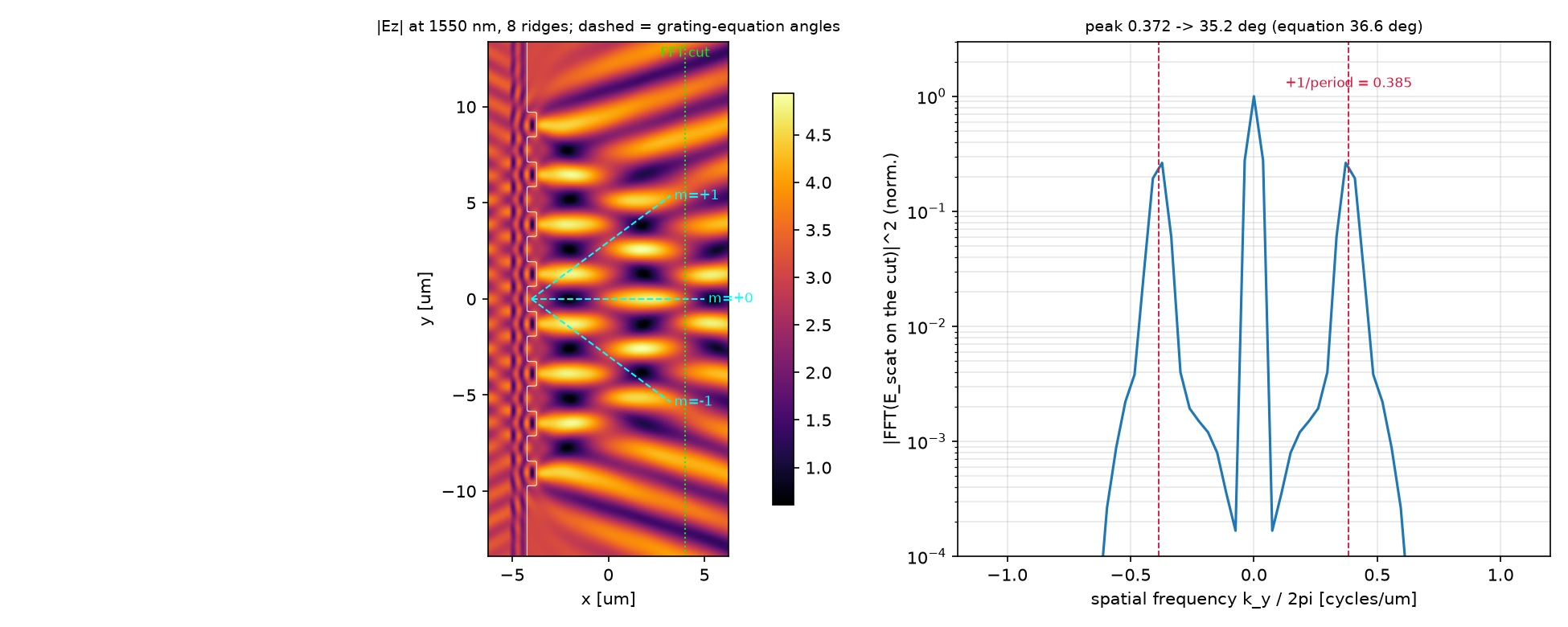
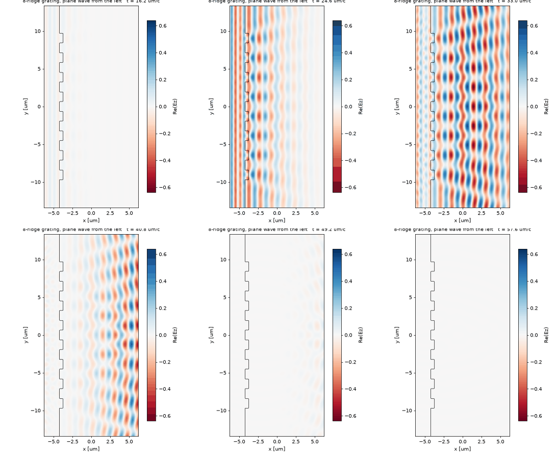
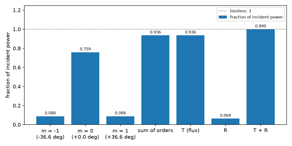
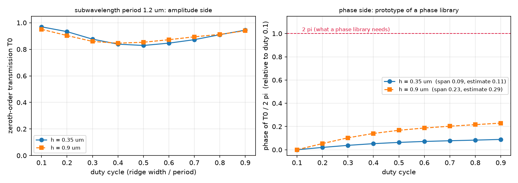
- Result: for a 2.6 µm period only m = 0, ±1 propagate (±36.6°). Power: m = 0 0.759, m = ±1 0.088 each; the orders add up to the transmitted flux and T + R = 0.999. The finite grating’s beams sit at 35.2° by spatial FFT. A duty-cycle sweep of a 1.2 µm period turns the phase by 0.09 × 2π (h = 0.35 µm) or 0.23 × 2π (h = 0.9 µm), close to Δn·h/λ.
- Takeaway: the grating equation fixes where the light can go; only a simulation says how much goes where. A single period with
k_pointis enough for the numbers, andDiffractedPlanewavedecomposes the transmitted field order by order. - Code: full script at the bottom, ~27 s on one core.
1. 관찰 · 빛의 경로를 먼저 보기
유리 막대 8개에 왼쪽에서 평면파를 보냈습니다. 막대 뒤에서 빛이 곧장 가는 방향과 비스듬히 가는 방향으로 나뉩니다. 청록 점선은 방정식으로 예측한 방향이고, 오른쪽 곡선은 실제 필드의 공간 FFT입니다.
2. 예측 · 결과를 읽기 전에
파장 1.55 µm에서 주기를 2.6 µm에서 1.2 µm로 줄이면, 공기 쪽으로 전파하는 ±1차 빔은 어떻게 될까요?
예측의 근거 확인하기
두 번째입니다. ±1차는 sin θ = ±λ/Λ를 만족해야 합니다. 1.55/1.2가 1보다 커 실수 각도가 없으므로 공기 중으로 멀리 전파하지 않습니다. 구조 가까이의 소멸장까지 사라진다는 뜻은 아닙니다.
3. 원리 이해하기 · 관찰을 설명하는 방법
방향은 주기와 파장으로 정한다
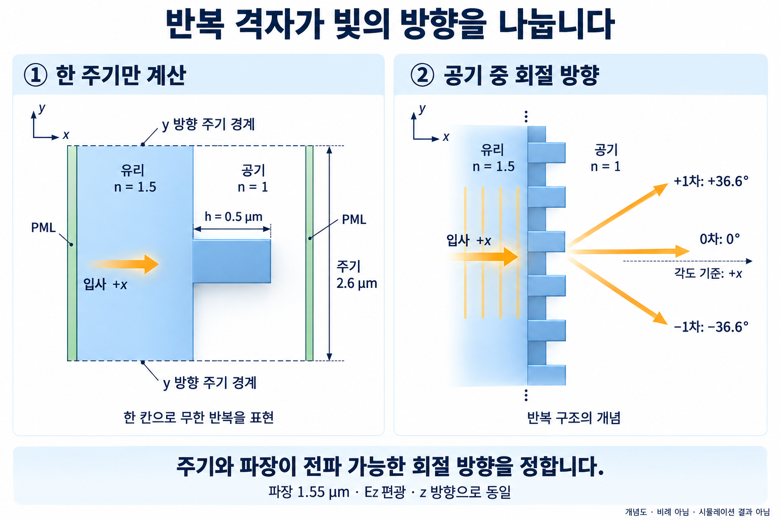
수직 입사한 빛이 공기로 나갈 때, 주기 Λ는 가로 방향 파수를 차수 m마다 다르게 만듭니다.
\[\sin\theta_m=m\lambda/\Lambda\]전파하려면 $\lvert m\rvert\lambda/\Lambda<1$이어야 합니다. 주기 2.6 µm와 파장 1.55 µm에서는 m = 0, ±1만 전파하고, ±1차 각도는 법선에서 ±36.6°입니다. 이 식은 갈 수 있는 방향을 알려주며 각 방향의 power는 알려주지 않습니다.
한 주기로 효율을 구하고 전체 합을 확인한다
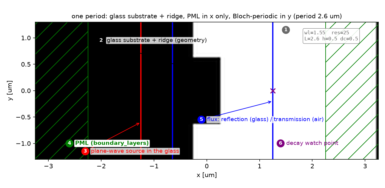
무한히 반복되는 격자는 막대 하나와 y 방향 주기 경계로 계산합니다. PML은 빛이 진행하는 x 방향에만 둡니다. DiffractedPlanewave로 각 차수의 복소 진폭을 분해한 뒤 입사 flux로 정규화합니다.
주기 1.2 µm에서는 0차만 전파합니다. 이때 duty cycle(막대 폭/주기)을 바꾸면 빔 개수보다 투과 진폭과 위상이 달라집니다. 유리의 낮은 굴절률 대비 때문에 높이 0.9 µm에서도 위상 변화는 한 바퀴에 못 미칩니다.
기호·설계 가정과 예측표 자세히 보기
주기 Λ의 구조는 평면파에 가로 방향 운동량 2πm/Λ를 더하거나 뺀다. 공기 중에서 전파하려면 가로 파수가 k₀ = 2π/λ보다 작아야 하므로 |m|λ/Λ < 1인 차수만 살아남는다. Λ = 2.6 µm, λ = 1.55 µm면 λ/Λ = 0.60이라 m = 0, ±1까지이고 ±1차는 ±36.6°로 간다. Λ = 1.2 µm면 λ/Λ = 1.29 > 1이라 0차만 남는다. 이때 격자는 “회절”하지 않고 하나의 유효 매질처럼 투과 진폭과 위상만 바꾼다.
\[\sin\theta_m=\frac{m\lambda}{\Lambda},\qquad T_m=\frac{\|a_m\|^2}{P_{\mathrm{in}}},\qquad \sum_m T_m = T_{\mathrm{total}},\qquad T_{\mathrm{total}}+R=1\] \[\frac{\Delta\phi_{\max}}{2\pi}\;\lesssim\;\frac{(n-1)\,h}{\lambda}\]두 번째 식은 duty cycle로 돌릴 수 있는 위상의 거친 상한이다. 높이 h의 막대를 지나며 쌓이는 위상차의 최대는 막대가 유리로 꽉 찼을 때와 비었을 때의 차, (n − 1)h/λ 바퀴다.
| 기호 | 뜻 | 코드 변수 |
|---|---|---|
| Λ, h, duty | 주기, 막대 높이, 막대 폭/주기 | gp, gh, gdc |
| $a_m$ | m차 평면파의 복소 진폭 (DiffractedPlanewave) |
amp[m] |
| $P_{\mathrm{in}}$ | reference run(유리로 꽉 찬 셀)의 투과 flux | P_in |
| $T_m$, R | m차 효율, 반사율(입사장 뺀 flux) | T_m[m], R |
| $k_y/2\pi$ | far cut 공간 FFT의 주파수 (cycles/µm) | ky |
가정과 유효 범위: 2D, Ez 편광, 수직 입사, 손실 없는 유리(n 1.5). 격자는 유리 기판 위의 유리 막대. 유한 격자의 각도는 FFT 분해능 1/(cut 길이) ≈ 0.037 cycles/µm(±1.8°)로 제한된다.
결과 보기 전에 맞춰보기
| 물리량 | 내 예측 | 근거 |
|---|---|---|
| 2.6 µm 주기의 전파 차수 | m = 0, ±1 세 개 | λ/Λ = 0.60 |
| ±1차 각도 | ±36.6° | asin(0.60) |
| T₊₁ = T₋₁ | 같음 | 수직 입사 + 대칭 막대 |
| ΣT_m과 T_total, T + R | 같음, 1 | 차수 분해 완비, 손실 없음 |
| 1.2 µm 주기의 T_total − T₀ | 0 | 0차만 전파 |
| duty cycle 위상 span (h 0.35 / 0.9 µm) | 0.11 / 0.29 × 2π 이하 | (n − 1)h/λ |
| 유한 격자 FFT 피크 | 0.385 cycles/µm (= 1/Λ) | 격자 방정식 |
판정 기준: ΣT_m이 T_total과 1%p 이상 다르면 차수 누락이나 DiffractedPlanewave 설정 오류. T + R이 1에서 1% 이상 벗어나면 reference run이 잘못됐다.
4. 직접 실행 · 변수 하나만 바꾸기
한 번만 바꿔보기: 회절 주기
- 전체 코드와
blogfig.py가 있는code/폴더에서python binary_grating.py를 실행하고 기준result.json을 보관합니다. GP_A, GH_A, GDC_A = 2.6, 0.5, 0.5에서 첫 값만 3.5로 바꿉니다. 높이·duty cycle·파장은 그대로 둡니다.- 다시 실행해
orders_propagating의 차수 목록, 각 차수의T_m, 그 합과T_total을 비교합니다.
방정식은 ±2차도 전파할 것으로 예측합니다. 새 차수에 얼마가 갈지는 계산으로 확인해야 합니다. 아래 측정 효율은 원래 2.6 µm 주기의 값이며, 3.5 µm의 효율은 새 실험 결과로 채워야 합니다. B 실험의 GP_B = 1.2는 그대로 유지합니다.
계산 배치·광원·파라미터 보기
| 파라미터 | 값 | 왜 이 값인가 | 바꾸면 |
|---|---|---|---|
| 주기 Λ (A / B) | 2.6 / 1.2 µm | A: m = 0, ±1만 전파하도록 공식 10 µm에서 축소. B: 0차만 | Λ ≥ 3.1 µm이면 ±2차도 생긴다 |
| 막대 h, duty (A) | 0.5 µm, 0.5 | 공식 예제 값 | 효율 배분이 바뀐다 (§7) |
fwidth |
0.1 fcen | 좁은 대역. 차수 분해는 한 주파수에서 | 넓히면 차수별 스펙트럼을 얻을 수 있다 |
RESOLUTION |
25 (수렴성 50) | 유리 안 파장 1.03 µm → 26 px, 막대 12 px | 50에서 소수 셋째 자리가 움직인다 |
| source | 유리 안, 셀 전체 폭 | 주기 셀에서는 폭 = 주기면 평면파 | — |
| reference run | 셀 전체가 유리 | 공식 예제 방식. P_in은 유리 안 입사 flux | 공기로 채우면 계면 반사가 분모에 들어간다 |
| 유한 격자 | ridge 8개, 공기 10 µm, 전면 PML | 빔이 분리될 거리. FFT cut은 막대 뒤 8 µm | ridge 수가 적으면 빔이 넓어진다 |
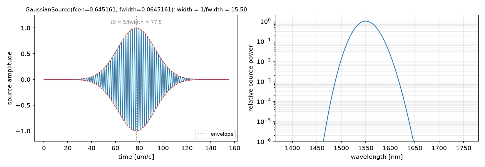
강의 노트북과의 차이: 강의 week 7은 1.2 µm 주기 하나로 duty cycle sweep을 하고 band 1 mode coefficient를 0차의 대리로 쓴다. 이 글은 공식 예제의 회절 주기(2.6 µm)에서 DiffractedPlanewave로 세 차수를 직접 분해하고, 수지 검산과 유한 격자 실험을 더했다. duty cycle sweep의 수치(위상 span 0.089 × 2π)는 강의와 같다.
코드 단계별 설명 보기
읽는 순서: 단위·파라미터 → 재료·구조 → source → Simulation·경계 → monitor → 실행·종료 → 후처리. 실험 A·B는 같은 함수
run_periodic로, 실험 C는 별도의 유한 셀로 돈다.
① 단위와 파라미터 — 어떤 숫자를 고정하는가
wl = 1.55
fcen = 1 / wl
fwidth = 0.1 * fcen           # narrow band: single-frequency order decomposition
n_glass = 1.5
glass = mp.Medium(index=n_glass)
DPML, DSUB, DPAD = 1.0, 2.0, 2.0

GP_A, GH_A, GDC_A = 2.6, 0.5, 0.5       # A: diffracting period (lambda / GP = 0.60 -> m = 0, +-1 only)
GP_B = 1.2                               # B: subwavelength period (lambda / GP = 1.29 -> m = 0 only)

def orders_propagating(gp):
    """Grating equation at normal incidence: sin(theta_m) = m * wl / gp (into air)."""
    m_max = int(np.floor(gp / wl))
    return {m: float(np.degrees(np.arcsin(m * wl / gp))) for m in range(-m_max, m_max + 1)}
- 무엇: 파장, 유리, 기판·공기 두께, 두 주기, 그리고 격자 방정식으로 전파 차수 목록을 미리 만든다.
- 왜: 어떤 차수를 분해할지는 시뮬레이션이 아니라 방정식이 정한다. 전파하지 않는 차수를
DiffractedPlanewave에 넣으면 소멸파라 의미 없는 수가 나온다. - 틀리면:
m_max를 잘못 세어 ±2차를 넣으면 그 진폭은 소멸파 성분이라 T_m 합이 T_total을 넘거나 들쭉날쭉해진다.
② 재료와 구조 — 무엇이 어디에 있는가
def grating_geometry(sx, gp, gh, gdc):
    return [mp.Block(material=glass, size=mp.Vector3(DPML + DSUB, mp.inf, mp.inf),
                     center=mp.Vector3(-0.5 * sx + 0.5 * (DPML + DSUB), 0)),          # substrate through the PML
            mp.Block(material=glass, size=mp.Vector3(gh, gdc * gp, mp.inf),
                     center=mp.Vector3(-0.5 * sx + DPML + DSUB + 0.5 * gh, 0))]      # the ridge, width gdc * gp
- 무엇: 왼쪽 PML을 관통하는 유리 기판과, 그 위의 막대 하나. 막대 폭이 duty × 주기다.
- 왜: 주기 셀에서는 막대 하나가 곧 무한 격자다. 기판은 PML을 관통해야 기판 뒷면 반사가 없다.
- 틀리면: 기판을 PML 앞에서 끊으면 유리·공기 계면이 하나 더 생겨 R에 4%가 추가된다.
③ Source — 빛을 어떻게 넣는가
def plane_wave(sx, sy, fw=fwidth):
    return [mp.Source(mp.GaussianSource(fcen, fwidth=fw), component=mp.Ez,
                      center=mp.Vector3(-0.5 * sx + DPML + 0.5 * DSUB, 0), size=mp.Vector3(0, sy))]
- 무엇: 유리 안에서 셀 전체 폭(= 한 주기)에 걸친 선원. +x로 가는 평면파다.
- 왜: 주기 경계 셀에서 셀 폭 전체의 선원은 그 자체로 무한 평면파다. 03편처럼
is_integrated가 필요 없다. y에는 PML이 없기 때문이다. - 틀리면: source를 공기 쪽에 두면 “유리 안 입사 flux” 정규화가 맞지 않는다.
④ Simulation과 경계 — 계산 상자와 PML
sim = mp.Simulation(cell_size=mp.Vector3(sx, gp), resolution=resolution,
                    boundary_layers=[mp.PML(DPML, direction=mp.X)],   # PML only along the propagation axis
                    geometry=[] if empty else grating_geometry(sx, gp, gh, gdc),
                    default_material=glass if empty else mp.air,     # reference: glass everywhere
                    sources=plane_wave(sx, gp), k_point=mp.Vector3())  # Bloch-periodic in y with k = 0
- 무엇: 높이가 한 주기뿐인 셀. PML은 x에만, y는
k_point=(0,0,0)의 Bloch 주기 경계. - 왜: 수직 입사면 Bloch 위상이 0이라
k_point가 영벡터다. reference run은 셀 전체를 유리로 채워 계면 없는 입사 flux를 잰다(공식 예제 방식). - 틀리면:
k_point를 빼면 y 경계가 반사벽이 되어 격자가 아니라 도파로를 계산한다. PML을 y에도 두면 주기성이 깨진다.
⑤ Monitor — 무엇을 재는가
refl = sim.add_flux(fcen, 0, 1, mp.FluxRegion(center=mp.Vector3(-0.5 * sx + DPML + 0.8 * DSUB, 0), size=mp.Vector3(0, gp)))
tran = sim.add_flux(fcen, 0, 1, mp.FluxRegion(center=mp.Vector3(0.5 * sx - DPML - 0.5 * DPAD, 0), size=mp.Vector3(0, gp)))
...
sim.load_minus_flux_data(refl, refl_data)     # reflection only (03편)
- 무엇: 유리 안의 반사 monitor(source 하류)와 공기 쪽의 투과 monitor. 둘 다 셀 폭 전체.
- 왜: 투과 monitor의 flux는 모든 차수의 합이고, 같은 monitor에서
DiffractedPlanewave로 차수를 나눈다. 반사 monitor는 03편 방식으로 입사장을 뺀다. - 틀리면: 투과 monitor를 막대에 너무 붙이면 소멸파 차수가 섞여 차수 합이 flux와 어긋난다. 막대에서 한 파장 이상 띄운다.
⑥ 실행과 종료 조건 — 언제 멈추는가
sim.run(until_after_sources=mp.stop_when_fields_decayed(50, mp.Ez, mp.Vector3(0.5 * sx - DPML - 0.5 * DPAD, 0), 1e-6))
- 무엇: 투과 monitor 위치의 Ez가 10⁻⁶으로 감쇠할 때까지.
- 왜: 좁은 대역이라 펄스가 길다(width 15.5). 꼬리까지 monitor를 지나야 DFT가 정확하다.
- 틀리면: 공식 예제처럼
until_after_sources=100고정 시간을 쓰면 다른 주기·높이에서 부족할 수 있다.
⑦ 후처리 — 숫자로 바꾸기
amp = {m: sim.get_eigenmode_coefficients(tran, mp.DiffractedPlanewave((0, m, 0), mp.Vector3(0, 1, 0), 1, 0)).alpha[0, 0, 0]
       for m in orders}                       # one order per call: (0, m, 0) along the periodic axis y, s-pol (Ez)
T_m = {m: abs(a) ** 2 / P_in for m, a in amp.items()}
phase_m = {m: np.angle(a) for m, a in amp.items()}
T_total = mp.get_fluxes(tran)[0] / P_in
R = -mp.get_fluxes(refl)[0] / P_in
- 무엇: 차수 m의 평면파 진폭 a_m을 하나씩 구해 |a_m|²/P_in을 효율로, 위각을 위상으로 쓴다.
- 왜:
DiffractedPlanewave((0, m, 0), axis, s, p)는 “주기 방향 y로 m번째 차수, s 편광(Ez)”이라는 하나의 평면파 모드다.get_eigenmode_coefficients는 이 객체를 한 번에 하나만 받는다. 04편의 band 번호 대신 차수를 직접 지정하는 셈이다. - 틀리면: 리스트로 여러
DiffractedPlanewave를 넘기면TypeError가 난다(처음 실행에서 그랬다).axis를 x로 주면 평면 정의가 바뀌어 s·p가 뒤집힌다.
함정: 위상 sweep은
np.unwrap으로 잇는다. 인접 표본의 위상차가 π보다 작을 때만 옳으므로 duty cycle을 촘촘히(9점) 잡는다. 이 글의 최대 인접 차는 0.33 rad이다.
5. 해석 · 측정값과 한계를 함께 읽기
방향 예측과 power 측정을 따로 읽기
| 차수 | 공기 중 각도 | 입사 power 대비 효율 |
|---|---|---|
| −1 | −36.6° | 0.0884 |
| 0 | 0° | 0.7591 |
| +1 | +36.6° | 0.0884 |
차수 합은 0.9358로 전체 투과 flux 0.9358과 맞고, R = 0.0635를 더하면 0.9994입니다. 대칭 구조·수직 입사이므로 ±1차가 같습니다. 해상도 50에서는 T₀ = 0.7597, T±1 = 0.0881로 바뀝니다.
주기 1.2 µm의 duty sweep은 높이 0.35/0.9 µm에서 각각 0.089/0.229 × 2π의 위상 범위를 줍니다. 높이가 커져도 여기서는 2π 전체를 덮지 못해 다음 편의 phase library 설계에 한계가 있습니다.
전체 측정표·예측 비교·수렴성 기록 보기
A. 2.6 µm 주기: 차수별 효율
| 양 | 값 (res 25) | 값 (res 50) | 10_sources 원본 (res 50) |
|---|---|---|---|
| T₀ | 0.7591 | 0.7597 | 0.7597 |
| T₊₁ = T₋₁ | 0.0884 | 0.0881 | 0.0881 |
| ΣT_m | 0.9358 | — | 0.9359 |
| T_total (flux) | 0.9358 | — | 0.9359 |
| R | 0.0635 | 0.0639 | 0.0639 |
| T + R | 0.9994 | 0.9998 | 0.9998 |
B. 1.2 µm 주기: duty cycle이 만드는 진폭과 위상
| 높이 h | 위상 span / 2π | 어림 (n − 1)h/λ | T₀ 범위 | max |T_total − T₀| |
|---|---|---|---|---|
| 0.35 µm | 0.089 | 0.113 | 0.83–0.97 | 3 × 10⁻⁶ |
| 0.90 µm | 0.229 | 0.290 | 0.85–0.95 | 3 × 10⁻⁶ |
C. 유한 격자: 빔과 각도
예측과 비교
| 물리량 | 내 예측 (§2) | 시뮬레이션 | 판정 |
|---|---|---|---|
| 전파 차수 | m = 0, ±1 | 세 차수의 합 = flux | ✅ |
| T₊₁ = T₋₁ | 같음 | 0.0884 = 0.0884 | ✅ |
| ΣT_m = T_total, T + R | 같음, 1 | 0.9358 = 0.9358, 0.9994 | ✅ |
| 1.2 µm의 T_total − T₀ | 0 | 3 × 10⁻⁶ | ✅ |
| 위상 span (0.35 / 0.9 µm) | ≤ 0.11 / 0.29 | 0.089 / 0.229 | ✅ |
| FFT 피크 | 0.385 cycles/µm | 0.372 (±0.037 분해능) | ✅ |
모두 맞았다. 위상 span은 어림의 79%다. 막대가 주기를 다 채우지 못하므로 유효 굴절률 차가 (n − 1)보다 작기 때문이고, 어림이 상한이라는 뜻이다. 높이를 2.6배 키워도 0.23바퀴다. 07편의 phase library가 유리 대신 Si를 쓰는 이유가 여기 있다.
수렴성
| resolution | T₀ | T₊₁ | R | T + R |
|---|---|---|---|---|
| 25 | 0.7591 | 0.0884 | 0.0635 | 0.9994 |
| 50 | 0.7597 | 0.0881 | 0.0639 | 0.9998 |
해상도를 2배 올려도 효율은 셋째 자리에서만 움직인다. 막대 높이 0.5 µm가 res 25에서 12 px라 충분하다.
주장할 수 있는 것 / 없는 것
- 할 수 있는 것: 이 격자에서 수직 입사 Ez 편광의 세 차수 효율은 0.76 / 0.088 / 0.088이고 수지가 닫힌다. subwavelength 유리 격자는 duty cycle로 위상을 (n − 1)h/λ 바퀴 이하만 돌린다.
- 할 수 없는 것: 유한 격자의 각도를 1° 안으로. FFT cut 길이가 ±1.8° 분해능을 정한다. 비스듬한 입사(Bloch 위상이 0이 아님)와 p 편광. 효율의 파장 의존성(한 주파수만 계산했다).
증상별 점검표 보기
| 증상 | 원인 | 고치는 법 |
|---|---|---|
TypeError ... DiffractedPlanewave |
여러 차수를 리스트로 넘김 | 차수마다 get_eigenmode_coefficients를 따로 호출 |
| 차수 합이 flux보다 큼 | 전파하지 않는 차수(소멸파)를 포함 | 격자 방정식으로 |m|λ/Λ < 1인 것만 |
| 격자가 도파로처럼 동작 | k_point 누락으로 y 경계가 반사벽 |
k_point=mp.Vector3() |
| R이 4%p 큼 | 기판이 PML 전에 끊김 | 기판 블록을 PML 관통 |
| 위상 곡선이 톱니 | unwrap 실패(표본 간격이 넓음) | duty cycle 점을 촘촘히 |
| 유한 격자 FFT 피크가 넓음 | cut이 짧거나 ridge 수가 적음 | cut 길이·ridge 수 늘리기 |
6. 확인 · 두 질문에 답해보기
1. 0차만 전파하면 막대가 빛에 아무 영향도 주지 않는 것일까요?
설명 확인하기
아닙니다. 멀리 전파하는 방향은 하나여도 0차의 진폭과 위상, 그리고 반사율이 바뀝니다. 이 복소 투과계수의 변화를 활용하는 것이 phase library의 출발점입니다.
2. ±1차 각도는 맞는데 차수 합이 전체 투과 flux와 다르면 무엇을 확인할까요?
설명 확인하기
전파하는 차수를 빠뜨렸거나 소멸 차수를 넣지 않았는지, DiffractedPlanewave의 주기 방향·편광 설정과 monitor 위치가 맞는지 확인합니다. 각도 방정식이 맞아도 효율 분해의 검산은 별도로 필요합니다.
7. 참고 · 전체 코드와 원본 기록
아래 전체 프로그램은 원본 그대로입니다. 실행 환경과 결과 기록을 함께 확인하세요.
binary_grating.py (클릭해서 펼치기)
"""Meep Example 06 - Binary grating and diffraction orders.

  A. One period of a glass binary grating (period 2.6 um > wavelength): the grating equation says only
     m = 0, +-1 propagate in air, at +-36.6 deg. DiffractedPlanewave gives the power in each order;
     checks: sum of orders = total transmitted flux, T + R = 1.  (official binary_grating.py, period reduced)
  B. A subwavelength period (1.2 um): only m = 0 propagates. Sweep the duty cycle and record the
     transmitted amplitude AND phase of the zeroth order, for two ridge heights. This curve is the
     prototype of the meta-atom phase library of post 07; the phase span scales like dn * h / lambda.
  C. A finite grating (8 ridges) with PML on all sides: the three beams become visible; the beam angle
     is read from the spatial FFT of the scattered field on a far cut and compared with the equation.
  D. GIF of C in time.

Run:  python binary_grating.py           (~5 min on one core)
Out:  00_source.png, 01_layout.png, 02_orders.png, 03_duty_sweep.png, 04_finite.png,
      05_anim_finite.gif, result.json   (-> ../assets/06/)
"""
import json
import os
import sys
import time

import numpy as np
import matplotlib
matplotlib.use("Agg")
import matplotlib.pyplot as plt
import meep as mp

sys.path.insert(0, os.path.dirname(os.path.abspath(__file__)))
from blogfig import Label, animate_fields, annotated_layout, bar_figure, record_frames, source_figure   # noqa: E402

OUT = os.path.join(os.path.dirname(os.path.abspath(__file__)), "..", "assets", "06")
os.makedirs(OUT, exist_ok=True)
t_all = time.time()

# ---------------------------------------------------------------- (1) units & parameters
wl = 1.55
fcen = 1 / wl
fwidth = 0.1 * fcen           # narrow band: single-frequency order decomposition
n_glass = 1.5
glass = mp.Medium(index=n_glass)
DPML, DSUB, DPAD = 1.0, 2.0, 2.0

GP_A, GH_A, GDC_A = 2.6, 0.5, 0.5       # A: diffracting period (lambda / GP = 0.60 -> m = 0, +-1 only)
GP_B = 1.2                               # B: subwavelength period (lambda / GP = 1.29 -> m = 0 only)
RESOLUTION = 25


def orders_propagating(gp):
    """Grating equation at normal incidence: sin(theta_m) = m * wl / gp (into air)."""
    m_max = int(np.floor(gp / wl))
    return {m: float(np.degrees(np.arcsin(m * wl / gp))) for m in range(-m_max, m_max + 1)}


# ---------------------------------------------------------------- (2) geometry: substrate + one ridge per period
def grating_geometry(sx, gp, gh, gdc):
    return [mp.Block(material=glass, size=mp.Vector3(DPML + DSUB, mp.inf, mp.inf),
                     center=mp.Vector3(-0.5 * sx + 0.5 * (DPML + DSUB), 0)),          # substrate through the PML
            mp.Block(material=glass, size=mp.Vector3(gh, gdc * gp, mp.inf),
                     center=mp.Vector3(-0.5 * sx + DPML + DSUB + 0.5 * gh, 0))]      # the ridge, width gdc * gp


# ---------------------------------------------------------------- (3) source: plane wave inside the glass, travelling +x
def plane_wave(sx, sy, fw=fwidth):
    return [mp.Source(mp.GaussianSource(fcen, fwidth=fw), component=mp.Ez,
                      center=mp.Vector3(-0.5 * sx + DPML + 0.5 * DSUB, 0), size=mp.Vector3(0, sy))]


# ---------------------------------------------------------------- (4) one periodic cell: PML in x only, Bloch-periodic in y (k = 0)
def periodic_cell(gp, gh, gdc, resolution=RESOLUTION, empty=False):
    sx = DPML + DSUB + gh + DPAD + DPML
    sim = mp.Simulation(cell_size=mp.Vector3(sx, gp), resolution=resolution,
                        boundary_layers=[mp.PML(DPML, direction=mp.X)],
                        geometry=[] if empty else grating_geometry(sx, gp, gh, gdc),
                        default_material=glass if empty else mp.air,     # reference: glass everywhere
                        sources=plane_wave(sx, gp), k_point=mp.Vector3())
    # ------------------------------------------------------------ (5) monitors: reflection (in glass), transmission (in air)
    refl = sim.add_flux(fcen, 0, 1, mp.FluxRegion(center=mp.Vector3(-0.5 * sx + DPML + 0.8 * DSUB, 0), size=mp.Vector3(0, gp)))
    tran = sim.add_flux(fcen, 0, 1, mp.FluxRegion(center=mp.Vector3(0.5 * sx - DPML - 0.5 * DPAD, 0), size=mp.Vector3(0, gp)))
    return sim, refl, tran, sx


def run_periodic(gp, gh, gdc, orders, resolution=RESOLUTION, layout=False):
    """Reference (all glass) then grating. Returns P_in-normalised T_m, T_total, R and the order amplitudes."""
    sim, refl, tran, sx = periodic_cell(gp, gh, gdc, resolution, empty=True)
    sim.run(until_after_sources=mp.stop_when_fields_decayed(50, mp.Ez, mp.Vector3(0.5 * sx - DPML - 0.5 * DPAD, 0), 1e-6))  # (6)
    P_in = float(mp.get_fluxes(tran)[0])                      # incident power per period (measured in glass)
    refl_data = sim.get_flux_data(refl)

    sim, refl, tran, sx = periodic_cell(gp, gh, gdc, resolution)
    sim.load_minus_flux_data(refl, refl_data)
    if layout:
        annotated_layout(
            sim, os.path.join(OUT, "01_layout.png"), dpml=DPML, figsize=(8.6, 4.2),
            title=f"one period: glass substrate + ridge, PML in x only, Bloch-periodic in y (period {gp} um)",
            params_text=f"wl={wl}  res={resolution}\nL={gp} h={gh} dc={gdc}",
            params_xy=(1.5, 1.15), pml_xy=(-2.6, -1.0), decay_point=(0.5 * sx - DPML - 0.5 * DPAD, 0), decay_text_xy=(1.4, -1.0),
            labels=[Label("glass substrate + ridge (geometry)", (-0.5 * sx + DPML + DSUB + 0.25, 0.3), (-2.0, 0.95), step=2, color="black"),
                    Label("plane-wave source in the glass", (-0.5 * sx + DPML + 0.5 * DSUB, -0.6), (-2.3, -1.15), step=3, color="red"),
                    Label("flux: reflection (glass) / transmission (air)", (0.5 * sx - DPML - 0.5 * DPAD, -0.2), (-0.1, -0.55), step=5, color="blue")],
            axis_step=1.0)
    sim.run(until_after_sources=mp.stop_when_fields_decayed(50, mp.Ez, mp.Vector3(0.5 * sx - DPML - 0.5 * DPAD, 0), 1e-6))
    # ------------------------------------------------------------ (7) orders by DiffractedPlanewave, totals by flux
    # one DiffractedPlanewave per call: order m along the periodic direction y, s-polarised (Ez)
    amp = {m: sim.get_eigenmode_coefficients(tran, mp.DiffractedPlanewave((0, m, 0), mp.Vector3(0, 1, 0), 1, 0)).alpha[0, 0, 0]
           for m in orders}
    T_m = {m: float(abs(a) ** 2 / P_in) for m, a in amp.items()}
    phase_m = {m: float(np.angle(a)) for m, a in amp.items()}
    return {"T_m": T_m, "phase_m": phase_m, "T_total": float(mp.get_fluxes(tran)[0] / P_in),
            "R": float(-mp.get_fluxes(refl)[0] / P_in), "P_in": P_in}


source_figure(fcen, fwidth, os.path.join(OUT, "00_source.png"), wl_scale=1000.0, wl_unit="nm", time_unit="um/c")

# ================================================================ A. diffraction orders of the 2.6 um grating
angles = orders_propagating(GP_A)
A = run_periodic(GP_A, GH_A, GDC_A, sorted(angles), layout=True)
sum_orders = sum(A["T_m"].values())
print(f"A. period {GP_A} um: propagating orders {sorted(angles)} at " + ", ".join(f"m={m}: {a:+.1f} deg" for m, a in sorted(angles.items())))
print(f"A. T_m = " + ", ".join(f"m={m}: {t:.4f}" for m, t in sorted(A['T_m'].items())) +
      f"; sum = {sum_orders:.4f}, T_total (flux) = {A['T_total']:.4f}, R = {A['R']:.4f}, T+R = {A['T_total'] + A['R']:.4f}")
bar_figure([f"m = {m}\n({angles[m]:+.1f} deg)" for m in sorted(angles)] + ["sum of orders", "T (flux)", "R", "T + R"],
           {"fraction of incident power": [A["T_m"][m] for m in sorted(angles)] + [sum_orders, A["T_total"], A["R"], A["T_total"] + A["R"]]},
           os.path.join(OUT, "02_orders.png"), ylabel="fraction of incident power", reference=1.0, reference_label="lossless: 1", figsize=(8, 4))
convergence = [{"resolution": RESOLUTION, **{f"T_{m}": A["T_m"][m] for m in sorted(angles)}, "R": A["R"], "T_plus_R": A["T_total"] + A["R"]}]
for res in (50,):
    Ar = run_periodic(GP_A, GH_A, GDC_A, sorted(angles), resolution=res)
    convergence.append({"resolution": res, **{f"T_{m}": Ar["T_m"][m] for m in sorted(angles)}, "R": Ar["R"], "T_plus_R": Ar["T_total"] + Ar["R"]})
    print(f"convergence res={res}: " + ", ".join(f"T_{m}={Ar['T_m'][m]:.4f}" for m in sorted(angles)) + f", R={Ar['R']:.4f}, T+R={Ar['T_total'] + Ar['R']:.4f}")

# ================================================================ B. subwavelength period: duty-cycle sweep of the zeroth order
duty = np.linspace(0.1, 0.9, 9)
sweep = {}
for gh in (0.35, 0.9):
    rows = [run_periodic(GP_B, gh, float(d), [0]) for d in duty]
    T0 = np.array([r["T_m"][0] for r in rows])
    ph = np.unwrap(np.array([r["phase_m"][0] for r in rows]))
    ph -= ph[0]
    step = float(np.max(np.abs(np.diff(ph))))
    sweep[gh] = {"duty": duty.tolist(), "T0": T0.tolist(), "phase": ph.tolist(), "span_over_2pi": float((ph.max() - ph.min()) / (2 * np.pi)),
                 "estimate_dn_h_over_wl": (n_glass - 1) * gh / wl, "max_step_rad": step,
                 "T_total_minus_T0_max": float(max(abs(r["T_total"] - r["T_m"][0]) for r in rows))}
    print(f"B. h={gh}: T0 in [{T0.min():.3f}, {T0.max():.3f}], phase span = {sweep[gh]['span_over_2pi']:.3f} x 2pi "
          f"(estimate dn*h/wl = {sweep[gh]['estimate_dn_h_over_wl']:.3f}), max step {step:.2f} rad, max|T_total - T0| = {sweep[gh]['T_total_minus_T0_max']:.1e}")
fig, ax = plt.subplots(1, 2, figsize=(11, 3.9))
for gh, st in ((0.35, "o-"), (0.9, "s--")):
    ax[0].plot(duty, sweep[gh]["T0"], st, label=f"h = {gh} um")
    ax[1].plot(duty, np.array(sweep[gh]["phase"]) / (2 * np.pi), st, label=f"h = {gh} um  (span {sweep[gh]['span_over_2pi']:.2f}, estimate {sweep[gh]['estimate_dn_h_over_wl']:.2f})")
ax[0].set_xlabel("duty cycle (ridge width / period)"); ax[0].set_ylabel("zeroth-order transmission T0"); ax[0].set_ylim(0, 1.05); ax[0].grid(alpha=0.3); ax[0].legend(fontsize=8)
ax[0].set_title(f"subwavelength period {GP_B} um: amplitude side", fontsize=9)
ax[1].axhline(1.0, color="crimson", ls="--", lw=1.0); ax[1].text(0.12, 1.02, "2 pi (what a phase library needs)", color="crimson", fontsize=8)
ax[1].set_xlabel("duty cycle"); ax[1].set_ylabel("phase of T0 / 2 pi  (relative to duty 0.1)"); ax[1].set_ylim(-0.05, 1.15); ax[1].grid(alpha=0.3); ax[1].legend(fontsize=8)
ax[1].set_title("phase side: prototype of a phase library", fontsize=9)
fig.tight_layout(); fig.savefig(os.path.join(OUT, "03_duty_sweep.png"), dpi=150); plt.close(fig)

# ================================================================ C. finite grating: the beams, and the angle from a spatial FFT
N_RIDGE = 8
RES_C = 15
pad_y = 3.0
sx_c = DPML + DSUB + GH_A + 10.0 + DPML
sy_c = N_RIDGE * GP_A + 2 * pad_y + 2 * DPML
x_ridge = -0.5 * sx_c + DPML + DSUB + 0.5 * GH_A


def finite_geometry(with_ridges):
    g = [mp.Block(material=glass, size=mp.Vector3(DPML + DSUB, mp.inf, mp.inf), center=mp.Vector3(-0.5 * sx_c + 0.5 * (DPML + DSUB), 0))]
    if with_ridges:
        for i in range(N_RIDGE):
            yc = (i - (N_RIDGE - 1) / 2) * GP_A
            g.append(mp.Block(material=glass, size=mp.Vector3(GH_A, GDC_A * GP_A, mp.inf), center=mp.Vector3(x_ridge, yc)))
    return g


def finite_sim(with_ridges, fw=fwidth, resolution=RES_C):
    return mp.Simulation(cell_size=mp.Vector3(sx_c, sy_c), resolution=resolution, boundary_layers=[mp.PML(DPML)],
                         geometry=finite_geometry(with_ridges),
                         sources=[mp.Source(mp.GaussianSource(fcen, fwidth=fw, is_integrated=True), component=mp.Ez,
                                            center=mp.Vector3(-0.5 * sx_c + DPML + 0.5 * DSUB, 0), size=mp.Vector3(0, sy_c))])


nonpml_c = mp.Volume(center=mp.Vector3(), size=mp.Vector3(sx_c - 2 * DPML, sy_c - 2 * DPML))
extent_c = [-(sx_c / 2 - DPML), sx_c / 2 - DPML, -(sy_c / 2 - DPML), sy_c / 2 - DPML]
fields = {}
for tag, ridges in (("flat", False), ("grating", True)):
    sim = finite_sim(ridges)
    dft = sim.add_dft_fields([mp.Ez], fcen, 0, 1, where=nonpml_c)
    sim.run(until_after_sources=mp.stop_when_fields_decayed(50, mp.Ez, mp.Vector3(0.5 * sx_c - DPML - 1.0, 0), 1e-5))
    fields[tag] = sim.get_dft_array(dft, mp.Ez, 0)
    if ridges:
        eps_c = sim.get_array(vol=nonpml_c, component=mp.Dielectric)
ez_sc = fields["grating"] - fields["flat"]                 # scattered field: what the ridges added
nx, ny = ez_sc.shape
xs = np.linspace(extent_c[0], extent_c[1], nx); ys = np.linspace(extent_c[2], extent_c[3], ny)
x_cut = x_ridge + 8.0                                      # far cut, 8 um past the ridges, in homogeneous air
line = ez_sc[np.argmin(abs(xs - x_cut)), :]
ky = np.fft.fftshift(np.fft.fftfreq(ny, d=ys[1] - ys[0]))  # cycles per um
spec = np.abs(np.fft.fftshift(np.fft.fft(line * np.hanning(ny)))) ** 2
spec /= spec.max()
pos = ky > 0.15
k_peak = float(ky[pos][np.argmax(spec[pos])])
theta_meas = float(np.degrees(np.arcsin(min(k_peak * wl, 1.0))))   # sin(theta) = k_y / k0 = k_peak * wl
print(f"C. finite grating ({N_RIDGE} ridges): spatial-FFT peak at {k_peak:.3f} cycles/um -> theta = {theta_meas:.1f} deg "
      f"(grating equation: 1/period = {1/GP_A:.3f} cycles/um -> {angles[1]:.1f} deg)")

fig, ax = plt.subplots(1, 2, figsize=(13, 5.2), gridspec_kw={"width_ratios": [1.5, 1]})
im = ax[0].imshow(np.abs(fields["grating"]).T, origin="lower", extent=extent_c, cmap="inferno", aspect="equal")
ax[0].contour(xs, ys, eps_c.T, levels=[0.5 * (eps_c.min() + eps_c.max())], colors="w", linewidths=0.5)
for m, a in angles.items():
    L = 9.0
    ax[0].plot([x_ridge, x_ridge + L * np.cos(np.radians(a))], [0, L * np.sin(np.radians(a))], "--", color="cyan", lw=1.0)
    ax[0].text(x_ridge + L * np.cos(np.radians(a)) + 0.2, L * np.sin(np.radians(a)), f"m={m:+d}", color="cyan", fontsize=8, va="center")
ax[0].axvline(x_cut, color="lime", ls=":", lw=1.0); ax[0].text(x_cut, extent_c[3] - 0.8, "FFT cut", color="lime", fontsize=8, ha="center")
ax[0].set_xlabel("x [um]"); ax[0].set_ylabel("y [um]"); ax[0].set_title(f"|Ez| at 1550 nm, {N_RIDGE} ridges; dashed = grating-equation angles", fontsize=9)
fig.colorbar(im, ax=ax[0], shrink=0.8)
ax[1].semilogy(ky, spec, color="tab:blue")
for m in (-1, 1):
    ax[1].axvline(m / GP_A, color="crimson", ls="--", lw=0.9)
ax[1].text(1 / GP_A, 1.2, f"+1/period = {1/GP_A:.3f}", color="crimson", fontsize=8, ha="center")
ax[1].set_xlim(-1.2, 1.2); ax[1].set_ylim(1e-4, 3); ax[1].set_xlabel("spatial frequency k_y / 2pi [cycles/um]"); ax[1].set_ylabel("|FFT(E_scat on the cut)|^2 (norm.)")
ax[1].set_title(f"peak {k_peak:.3f} -> {theta_meas:.1f} deg (equation {angles[1]:.1f} deg)", fontsize=9); ax[1].grid(alpha=0.3, which="both")
fig.tight_layout(); fig.savefig(os.path.join(OUT, "04_finite.png"), dpi=150); plt.close(fig)

# ================================================================ D. GIF: the beams forming in time
fw_anim = 0.3 * fcen
sim_anim = finite_sim(True, fw=fw_anim, resolution=12)
sim_anim.init_sim()
eps_anim = sim_anim.get_array(vol=nonpml_c, component=mp.Dielectric)
frames, times = record_frames(sim_anim, nonpml_c, mp.Ez, t_start=5 / fw_anim - 2 / fw_anim, t_end=5 / fw_anim + 1.5 * sx_c + 10, n_frames=60)
animate_fields(frames, times, extent_c, os.path.join(OUT, "05_anim_finite.gif"), eps=eps_anim, figsize=(5.2, 6.4), dpi=70,
               title=f"{N_RIDGE}-ridge grating, plane wave from the left", legend_loc="lower right")

if mp.am_master():
    with open(os.path.join(OUT, "result.json"), "w") as f:
        json.dump({"A": {"period": GP_A, "angles_deg": angles, **{k: A[k] for k in ("T_m", "phase_m", "T_total", "R")}, "sum_orders": sum_orders},
                   "convergence": convergence, "B": {str(k): v for k, v in sweep.items()},
                   "C": {"n_ridges": N_RIDGE, "k_peak_cycles_per_um": k_peak, "theta_meas_deg": theta_meas, "theta_eq_deg": angles[1]},
                   "wall_s_total": time.time() - t_all, "meep": mp.__version__}, f, indent=2)
원본 실행 로그·재현 환경 보기
§4의 발췌 코드와 달리 전체 코드에는 유한 격자 실험(C), 그림 저장·GIF 녹화·result.json 기록이 들어 있다. 그림 helper blogfig.py는 시리즈 공통이며 같은 폴더(code/)에 있다. 전체 코드와 helper: https://github.com/jin-castle/meep-examples/blob/main/code.
실행 결과 (2026-10-23 실행):
A. period 2.6 um: propagating orders [-1, 0, 1] at m=-1: -36.6 deg, m=0: +0.0 deg, m=1: +36.6 deg
A. T_m = m=-1: 0.0884, m=0: 0.7591, m=1: 0.0884; sum = 0.9358, T_total (flux) = 0.9358, R = 0.0635, T+R = 0.9994
convergence res=50: T_-1=0.0881, T_0=0.7597, T_1=0.0881, R=0.0639, T+R=0.9998
B. h=0.35: T0 in [0.829, 0.969], phase span = 0.089 x 2pi (estimate dn*h/wl = 0.113), max step 0.13 rad, max|T_total - T0| = 2.6e-06
B. h=0.9: T0 in [0.846, 0.950], phase span = 0.229 x 2pi (estimate dn*h/wl = 0.290), max step 0.33 rad, max|T_total - T0| = 2.6e-06
C. finite grating (8 ridges): spatial-FFT peak at 0.372 cycles/um -> theta = 35.2 deg (grating equation: 1/period = 0.385 cycles/um -> 36.6 deg)
재현 환경: meep 1.33.0 · Python 3.11 · conda install -c conda-forge pymeep · 실행 python binary_grating.py (약 27 s, 단일 코어)
응용과 다음 학습 주제 보기
어디에 쓰이는가
회절 격자는 분광기, 광섬유 결합기, AR 안경, 홀로그램의 공통 부품이다. 차수별 효율이 그 부품의 성능이다.
| 응용 | 이 글의 어떤 것을 쓰는가 | 그 다음에 필요한 것 |
|---|---|---|
| 분광기·모노크로미터 | 차수별 효율, grating equation | 16편 far field |
| grating coupler(광섬유 ↔ 칩) | 차수 하나로 몰기, 각도 | 07편 meta-atom |
| AR 안경의 도파로 격자, 홀로그램, 회절 광학소자(DOE) | duty cycle이 만드는 위상 | 07편 phase library |
| 유한한 격자의 빔 각도 | FFT로 잰 회절 각도 | 16편 |