MEEP EXAMPLES 07
막대의 폭만 바꿔 빛의 방향을 정할 수 있을까?
Si 막대의 폭을 위상으로 바꾸는 표를 만들고, 네 막대를 골라 빛을 기울입니다. 단위 셀의 예상과 실제 배열의 효율 사이에 왜 차이가 남는지 확인합니다.
이 글을 읽고 나면
- 복소 투과계수의 진폭과 위상으로 phase library를 읽는다.
- 네 단계의 위상 배열과 목표 회절 각도를 연결한다.
- 실제 효율을 이상적 상한 및 해상도 오차와 구분한다.
먼저 알면 좋은 것 06편의 주기 셀·회절 차수·duty cycle 위상을 알면 좋습니다. 실행에는 Meep와 Python이 필요합니다.
English summary
- What: a silicon bar in a 0.45 µm unit cell is a meta-atom. Sweep its width, record the complex transmission t(w), and you have a phase library. Pick four widths that step the phase by 90°, tile them into a 1.8 µm supercell, and the structure should deflect 1550 nm light to +59.4°.
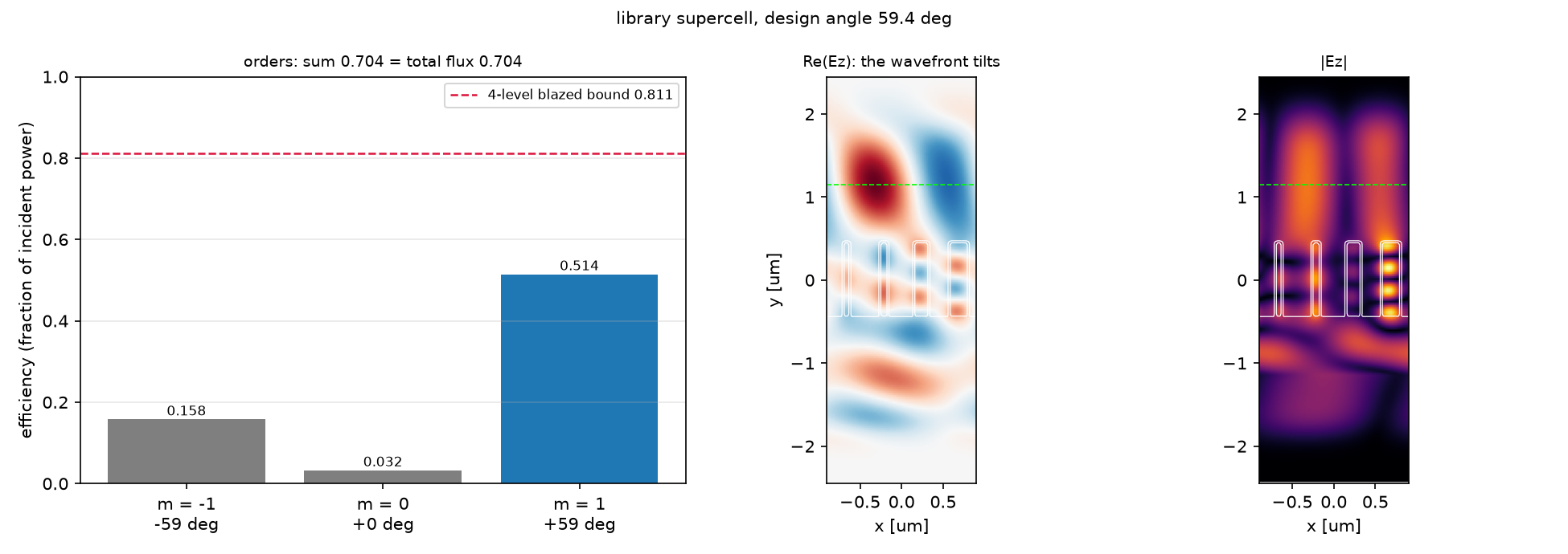
- Result: the library covers 1.10 × 2π with |t| between 0.69 and 1.01. The 4-level supercell sends 51 % of the power into the +1 order, 16 % into −1 and 3 % straight through; that is 63 % of the 4-level blazed bound 0.81. A 40-atom array peaks at 58.5°.
- Takeaway: the library assumes every neighbour is identical. In the real supercell they are not, so the local-phase approximation leaks power into the wrong orders. That gap is what inverse design (post 08) closes.
- Code: full script at the bottom, ~35 s on one core.
1. 관찰 · 빛의 경로를 먼저 보기
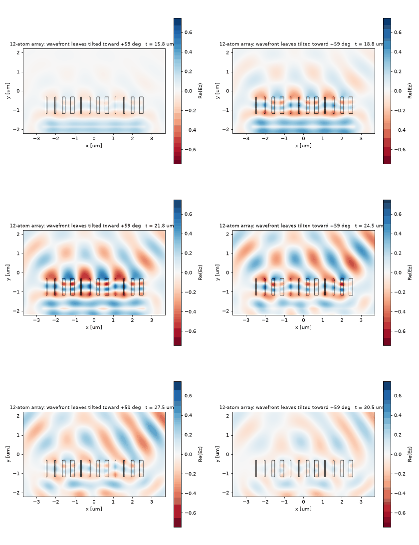
폭이 다른 네 Si 막대를 반복해 배치했습니다. 빛은 아래에서 위로 들어오고, 막대를 지난 파면은 오른쪽으로 기웁니다. 오른쪽으로 나가는 +1차에 모든 빛이 모였는지 왼쪽 차수별 효율 막대그래프로 확인해 보세요.
2. 예측 · 결과를 읽기 전에
단위 셀의 위상이 2π 전체를 덮으면, 네 막대를 조합한 배열도 반드시 목표 차수로 100% 보낼까요?
예측의 근거 확인하기
두 번째입니다. 위상을 네 단계로 근사하는 것만으로도 이상적 모델의 효율은 약 0.811입니다. 실제 막대의 진폭은 같지 않고, 단위 셀에서 가정했던 동일한 이웃도 실제 배열에서는 달라집니다. 따라서 2π 커버는 필요한 설계 조건이지 100% 효율 보장이 아닙니다.
3. 원리 이해하기 · 관찰을 설명하는 방법
폭을 위상으로 바꾸는 표가 phase library다
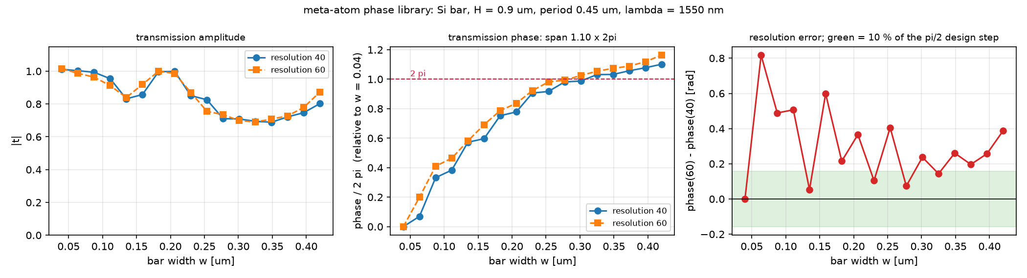
주기 0.45 µm의 단위 셀은 1550 nm에서 0차만 전파합니다. 한 주기 위의 복소 DFT 필드를 평균하고 막대 없는 셀로 나누면 복소 투과계수 t(w)를 얻습니다. 그 크기는 진폭, 위각은 위상입니다. 폭을 바꾸며 두 값을 기록한 표가 library입니다.
\[t(w)=\frac{\langle E_z\rangle(w)}{\langle E_z\rangle(0)}\]위상은 np.unwrap으로 이어 읽지만, 표본 사이의 실제 변화가 너무 크면 제대로 복원할 수 없습니다. 진폭이 크게 떨어지는 폭도 함께 확인해야 합니다. 여기의 t는 막대 없는 기준 셀 대비 필드 비율이므로 그 크기 자체를 입사 power 대비 효율로 읽지 않습니다.
네 개의 폭으로 기울어진 파면을 만든다
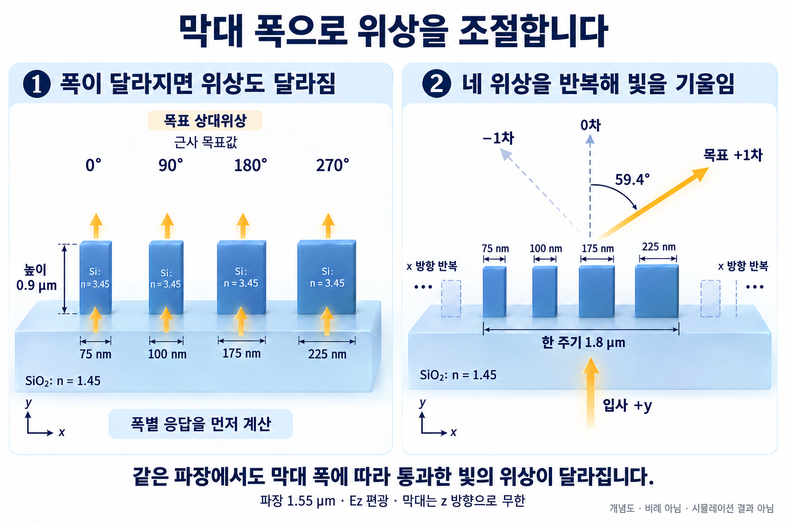
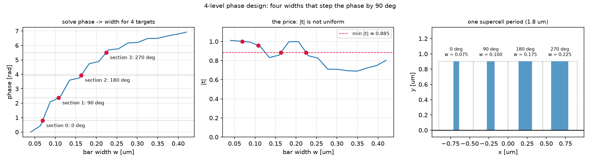
네 구획의 목표 상대위상은 0°, 90°, 180°, 270°입니다. 시작 위상 φ₀를 함께 이동해도 위상 기울기는 같으므로 목표 각도는 유지됩니다. 이 자유도로 진폭이 너무 작은 폭을 피합니다.
\[\Lambda=4\times0.45=1.8\;\mu\mathrm{m},\qquad \sin\theta_{+1}=1.55/1.8\]목표 각도는 +y 법선에서 오른쪽으로 59.4°입니다. 실제 선택 폭은 75, 100, 175, 225 nm입니다. 각 막대를 고를 때의 library는 같은 폭의 이웃이 무한히 반복되는 조건이며, 서로 다른 폭을 이웃으로 놓는 순간 그 근사가 검증 대상이 됩니다.
기호·설계 가정과 예측표 자세히 보기
주기 Λ_a = 0.45 µm(파장의 0.29배)의 unit cell에 든 Si 막대는 회절하지 않는다. 0차만 전파하므로 unit cell 전체가 복소 투과계수 t(w) 하나로 요약된다. 막대가 넓을수록 유효 굴절률이 커져 위상이 더 쌓인다. 높이 H = 0.9 µm, Δn ≈ 2.45로 어림 Δn·H/λ = 1.4바퀴이니 한 바퀴는 넘길 수 있다.
+1차로 꺾으려면 투과 위상이 x에 비례해 φ(x) = 2πx/Λ여야 한다. Λ = 4Λ_a = 1.8 µm로 두고 네 구획에 0°, 90°, 180°, 270°를 주면 계단식 근사가 된다. N단계로 이산화한 blazed 격자의 +1차 효율 상한은 sinc²(1/N)이고 N = 4면 0.81이다. 그 위에 두 가지 손실이 더 얹힌다. |t|가 균일하지 않은 것, 그리고 library가 “이웃이 모두 나와 같다”는 주기 가정에서 나온 값이라 폭이 다른 이웃 옆에서는 틀린다는 것.
\[t(w)=\frac{\langle E_z\rangle_{\text{period}}(w)}{\langle E_z\rangle_{\text{period}}(0)},\qquad \phi_{\text{target}}(x)=\frac{2\pi x}{\Lambda},\qquad \sin\theta_{+1}=\frac{\lambda}{\Lambda}=\frac{1.55}{1.8}\Rightarrow 59.4^\circ,\qquad \eta_{+1}\le\mathrm{sinc}^2\!\Big(\frac1N\Big)=0.811\]| 기호 | 뜻 | 코드 변수 |
|---|---|---|
| Λ_a, Λ | atom 주기 0.45, supercell 주기 1.8 µm | LA, LAMBDA |
| w, H | 막대 폭(설계 변수), 높이 0.9 µm | widths, H |
| t(w) | 빈 셀로 정규화한 0차 복소 투과 | t_atom(w) / t_atom(0) |
| φ₀ | 네 목표 위상의 시작점(전역 위상) | phi0 |
| w_lib | 선택된 네 폭(픽셀 정렬) | w_lib |
| η_m | m차 효율 (입사 flux 대비) | orders[m]["eff"] |
| θ_d | 설계 편향각 59.44° | THETA_D |
가정과 유효 범위: 2D, Ez 편광, 수직 입사, 손실 없는 Si(3.45)·SiO₂(1.45). library는 res 40에서 만들고 res 60과 비교한다. far field는 2D 선 초점의 각도 분포다.
결과 보기 전에 맞춰보기
| 물리량 | 내 예측 | 근거 | ||
|---|---|---|---|---|
| 위상 span (H 0.9, Si) | 1바퀴 이상 | Δn·H/λ = 1.4의 70~80% (06편 경험) | ||
| 위상의 단조성 | w에 대해 단조 증가 | 넓을수록 유효 굴절률 증가 | ||
| |t| | 넓은 w에서 떨어짐 | 막대 공명·반사 | ||
| +1차 효율 | 0.81 미만, 0.5~0.7 | 4단계 상한 × | t | 불균일 × 이웃 결합 |
| −1차와 0차 | 0은 아님, 합쳐 0.1~0.2 | 계단 근사의 누설 | ||
| 40-atom 빔 방향 | 59° 근처, 10-atom은 더 벗어남 | 개구가 짧으면 빔폭이 커지고 피크가 밀린다 |
판정 기준: 차수 합이 총 투과 flux와 1%p 이상 다르면 분해 오류. 위상 unwrap에서 인접 차가 π를 넘으면 표본 부족.
4. 직접 실행 · 변수 하나만 바꾸기
한 번만 바꿔보기: 설계 해상도
meta_atom.py와blogfig.py가 있는code/폴더에서python meta_atom.py를 실행합니다. 기준result.json의 선택 폭 네 개와 +1차 효율을 보관합니다.RES = 40을RES = 60으로만 바꾸고 다시 실행합니다. 폭 표본 17개 전체와 다른 구조·파라미터는 유지합니다.- 새 library에서 고른 폭과 supercell의 +1차 효율을 원본과 비교합니다. 두 경우 모두 차수 합이 총 투과 flux와 맞는지도 확인합니다.
원본에는 해상도 60의 library 비교가 있지만, 그 library로 다시 설계한 배열의 효율은 기록되어 있지 않습니다. 그 값을 새 실험에서 구합니다. 일부 폭만 재계산하면 unwrap의 branch가 달라질 수 있으므로 표본 전체를 사용합니다.
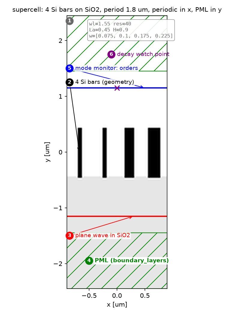
계산 배치·광원·파라미터 보기
| 파라미터 | 값 | 왜 이 값인가 | 바꾸면 |
|---|---|---|---|
| Λ_a | 0.45 µm | res 40에서 정확히 18 px. 픽셀 정수가 아니면 Meep이 셀을 반올림해 실제 주기와 k_x = m/Λ가 어긋난다 | θ_d가 따라 바뀐다 |
| Λ = 4Λ_a, θ_d | 1.8 µm, 59.44° | θ_d를 먼저 정하지 않고 주기를 픽셀 정수로 고정한 뒤 각도가 따라오게 | — |
| H | 0.9 µm | 2π를 넘기는 최소 높이 근처 | 낮추면 span < 2π |
widths |
0.04–0.42, 17점 | unwrap 조건(인접 차 < π)을 만족하는 밀도 | 성기면 unwrap이 2π 틀린다 |
RES |
40 (수렴성 60) | 폭 0.075 µm 막대가 3 px | 60에서 위상이 최대 0.82 rad 바뀐다(§5) |
| 종료 | monitor 점 Ez 1e-7 감쇠 | 좁은 대역(fwidth 0.1 fcen) 펄스 꼬리 | 고정 시간이면 폭마다 다르게 틀린다 |
| far field | R = 200 µm, 341각, source는 배열 폭만 | 배열 옆 빈 구간의 빛이 0° 인공물이 되지 않게 | 셀 전체 폭 source면 0°가 과대 |
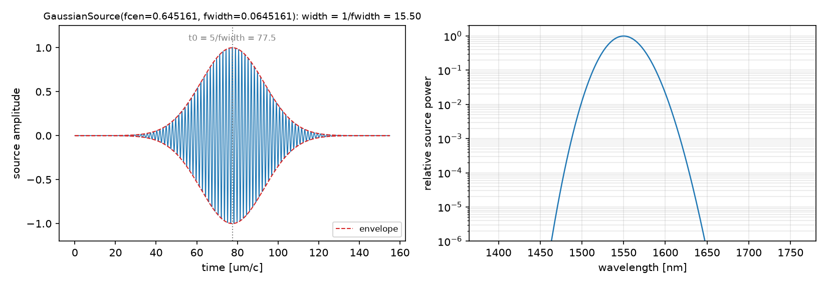
강의 노트북과의 차이: 없다. 파라미터·절차·수치 모두 강의 week 8과 같다(위상 span 1.101 × 2π, 설계 폭 네 개, +1차 0.514). 이 글은 거기에 10_sources의 공식 metasurface_lens 재현에서 얻은 두 가지 주의(wrapped phase를 그대로 불연속으로 읽지 말 것, 목표 위상을 library와 같은 2π branch에 둘 것)를 §4·§6에 덧붙였다.
코드 단계별 설명 보기
읽는 순서: 단위·파라미터 → 재료·구조 → source → Simulation·경계 → monitor → 실행·종료 → 후처리. 전파 방향이 +y라서 06편과 x·y가 바뀐다. 실험 A(library)는 unit cell, C(supercell)는 네 배 넓은 셀, D(far field)는 PML 전면의 유한 셀이다.
① 단위와 파라미터 — 어떤 숫자를 고정하는가
wl = 1.55; fcen = 1 / wl; fwidth = 0.1 * fcen
Si, SiO2 = mp.Medium(index=3.45), mp.Medium(index=1.45)
N_SEC = 4                       # phase levels per supercell period
LA = 0.45                       # atom period [um]: 18 px at resolution 40
LAMBDA = N_SEC * LA             # supercell period 1.80 um
THETA_D = np.degrees(np.arcsin(wl / LAMBDA))   # 59.44 deg
H = 0.9                         # bar height [um]
RES = 40
DPML, DSUB, DAIR = 1.0, 1.0, 1.0
SY = DPML + DSUB + H + DAIR + DPML
Y_BOT = -0.5 * SY; Y_DEV = Y_BOT + DPML + DSUB; SRC_Y = Y_BOT + DPML + 0.3; MON_Y = -Y_BOT - DPML - 0.3
BLAZED_BOUND = (np.sin(np.pi / N_SEC) / (np.pi / N_SEC)) ** 2   # 0.8106
- 무엇: atom 주기를 픽셀 정수로 먼저 고정하고, supercell 주기와 편향각을 거기서 유도한다. blazed 상한도 여기서 계산해 둔다.
- 왜: θ_d = 60°로 잡으면 Λ = 1.7898 µm로 픽셀 정수가 아니다. Meep이 셀을 반올림하면 “주기”와 차수 계산 k_x = m/Λ가 어긋난다. 숫자를 먼저 고정하고 각도가 따라오게 하면 이 문제가 없다.
- 틀리면: 셀 반올림 경고가 뜨고 ±1차의 각도·효율이 미세하게 틀린다. 06편에서 1.2 µm 주기가 res 22에서 반올림된 것도 같은 문제였다.
② 재료와 구조 — 무엇이 어디에 있는가
def geometry_bars(widths, period):
    g = [mp.Block(center=mp.Vector3(0, Y_BOT + 0.5 * (DPML + DSUB)), size=mp.Vector3(mp.inf, DPML + DSUB), material=SiO2)]
    n = len(widths)
    for j, w in enumerate(widths):
        if w > 0:
            xj = -0.5 * period + (j + 0.5) * period / n
            g.append(mp.Block(center=mp.Vector3(xj, Y_DEV + 0.5 * H), size=mp.Vector3(w, H), material=Si))
    return g
- 무엇: 기판 위에 구획마다 Si 막대 하나.
widths=[w]면 unit cell,widths=w_lib면 4구획 supercell이다. - 왜: library와 supercell이 같은 함수로 만들어져야 “library 값을 그대로 썼는데 왜 다른가”를 물을 수 있다. w = 0은 막대 없는 reference다.
- 틀리면: 막대 중심을 구획 중심에 두지 않으면 위상 기울기에 오프셋이 생겨 0차가 커진다.
③ Source — 빛을 어떻게 넣는가
def plane_wave(period, fw=fwidth, integrated=False):
    return [mp.Source(mp.GaussianSource(fcen, fwidth=fw, is_integrated=integrated), component=mp.Ez,
                      center=mp.Vector3(0, SRC_Y), size=mp.Vector3(period, 0))]
- 무엇: 기판 안에서 셀 폭 전체의 가로선. +y로 가는 평면파.
- 왜: 주기 셀에서는 셀 폭 = 주기라 그 자체로 평면파다. 유한 배열(D)에서만
is_integrated=True와 “배열 폭만큼”의 선원을 쓴다. - 틀리면: 유한 배열에서 셀 전체 폭으로 쏘면 배열 옆 빈 기판을 그대로 통과한 빛이 0° 피크로 크게 섞인다.
④ Simulation과 경계 — 계산 상자와 PML
def periodic_sim(widths, period, resolution=RES):
    return mp.Simulation(resolution=resolution, cell_size=mp.Vector3(period, SY), geometry=geometry_bars(widths, period),
                         boundary_layers=[mp.PML(thickness=DPML, direction=mp.Y)], k_point=mp.Vector3(),
                         sources=plane_wave(period))
- 무엇: PML은 y에만, x는
k_point=0의 주기 경계. 06편과 축만 다르다. - 왜: unit cell의 t(w)는 “무한 주기 배열 안의 막대”의 값이다. 이 가정이 뒤에서 깨지는 지점을 보게 된다.
- 틀리면: unit cell에 PML을 x에도 두면 고립된 막대 하나의 산란을 계산하게 되고 t(w)의 의미가 달라진다.
⑤ Monitor — 무엇을 재는가
# A. unit cell: DFT of Ez on a line across one period; its mean is the zeroth Fourier coefficient
dft = sim.add_dft_fields([mp.Ez], fcen, 0, 1, center=mp.Vector3(0, MON_Y), size=mp.Vector3(LA, 0))
t = np.mean(sim.get_dft_array(dft, mp.Ez, 0))
# C. supercell: a mode monitor across the period, decomposed order by order
mon = sim.add_mode_monitor(fcen, 0, 1, mp.ModeRegion(center=mp.Vector3(0, MON_Y), size=mp.Vector3(LAMBDA, 0)))
a_m = sim.get_eigenmode_coefficients(mon, mp.DiffractedPlanewave((m, 0, 0), mp.Vector3(1, 0, 0), 1, 0)).alpha[0, 0, 0]
- 무엇: unit cell에서는 한 주기 위의 복소 DFT를 평균해 t를 얻고, supercell에서는 06편처럼 차수별 진폭을 얻는다.
- 왜: 주기 함수의 한 주기 평균은 0차 Fourier 계수다. subwavelength 셀에서는 0차만 전파하므로 평균 하나가 투과 전부다.
get_array가 아니라get_dft_array인 이유는 마지막 시각의 snapshot이 아니라 정상상태 복소 진폭이 필요하기 때문이다. - 틀리면:
get_array로 재면 펄스가 지나간 뒤의 잔재를 평균하게 된다. monitor를 막대 바로 위에 두면 소멸파가 섞인다(여기서는 0.7 µm 위).
⑥ 실행과 종료 조건 — 언제 멈추는가
sim.run(until_after_sources=mp.stop_when_fields_decayed(10, mp.Ez, mp.Vector3(0, MON_Y), 1e-7))
- 무엇: monitor 점의 Ez가 10⁻⁷로 줄 때까지. 34번의 library run 모두 같은 조건.
- 왜: 복소 위상은 진폭보다 꼬리에 민감하다. 임계값을 보통(10⁻⁶)보다 낮게 둔다.
- 틀리면: 폭마다 종료 시각이 달라져도 상관없지만, 고정 시간으로 끊으면 어떤 폭에서는 꼬리가 남아 위상이 틀어진다.
⑦ 후처리 — 숫자로 바꾸기
t_ref = t_atom(0.0)
t = np.array([t_atom(w) / t_ref for w in widths])
phase = np.unwrap(np.angle(t)); phase -= phase[0]          # library: |t|, relative phase

# design: for each trial phi0, four targets phi0 + k*pi/2 -> widths by inverse interpolation; keep the phi0 with the largest min|t|
targets = phi0 + np.arange(N_SEC) * (2 * np.pi / N_SEC)
ws = np.interp(targets, ph_dense, w_dense)
w_lib = np.round(ws * RES) / RES                            # snap to the pixel grid

eff_m = abs(a_m) ** 2 / P_in                               # supercell: efficiency per order, P_in from an all-SiO2 run
- 무엇: 빈 셀로 나눈 t의 위상을 unwrap해 library를 만들고, 목표 위상에서 폭을 역으로 읽으며, 전역 위상 φ₀를 골라 min|t|를 키운다. 폭은 픽셀에 맞춘다.
- 왜:
np.angle은 (−π, π]의 wrapped 값이다. 10_sources의 phase map 노트가 경고하듯, 거기서 보이는 급변은 물리적 불연속이 아니라 branch cut일 수 있다. unwrap은 인접 표본의 차가 π보다 작을 때만 옳으므로 폭을 촘촘히 잡았다. library의 위상은 상대값이라 상수를 더해도 되고, 그 자유도가 |t| 균일성을 사는 데 쓰인다. - 틀리면: 목표 위상을 library와 다른 2π branch에 두고 clip하면 네 폭이 모두 library 최솟값으로 몰린다(10_sources 실패 사례). 픽셀 정렬을 빼면 supercell 막대 폭이 library와 다른 값으로 반올림된다.
함정: 성긴 폭 부분집합만 다시 돌려 수렴성을 보면 unwrap이 어긋나 2π만큼 틀린다. 수렴성 비교는 같은 폭 격자 전체로 library를 다시 만든 뒤 한다(§5).
5. 해석 · 측정값과 한계를 함께 읽기
위상 한 바퀴와 효율 100%는 다르다
원본 library는 위상 1.101 × 2π를 덮고, 진폭 범위는 0.689–1.011입니다. 선택 폭의 진폭은 1.001, 0.959, 0.885, 0.885로 균일하지 않습니다.
| 실제 supercell의 차수 | 각도 | 입사 flux 대비 효율 |
|---|---|---|
| −1 | −59.4° | 0.1576 |
| 0 | 0° | 0.0325 |
| +1 | +59.4° | 0.5144 |
합 0.7045는 전체 투과 flux와 일치합니다. 목표 차수의 0.5144는 이상적 4단계 모델 0.8106의 63.5%입니다. 이 차이를 진폭 불균일과 이웃 결합으로 각각 얼마씩 나눌지는 이 실험만으로 알 수 없습니다.
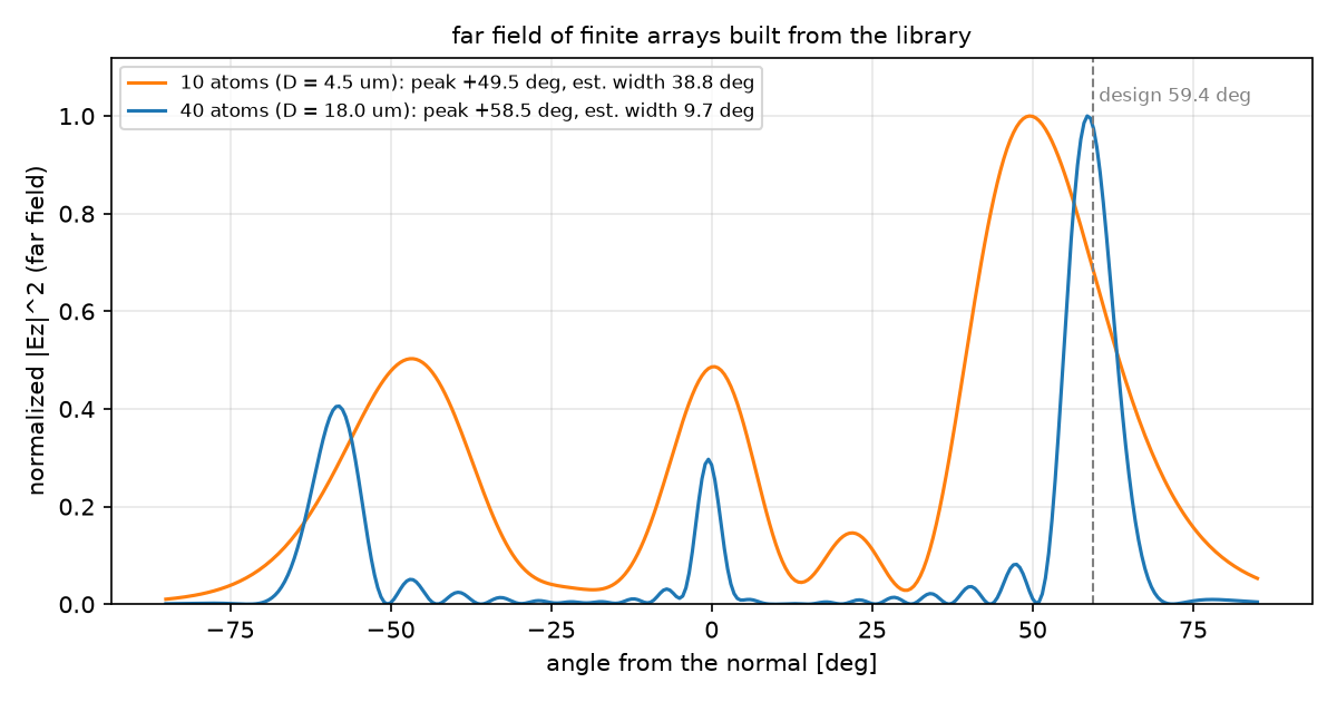
유한 배열에서는 개구도 중요합니다. 10개 막대(4.5 µm)의 피크는 49.5°, 40개(18 µm)는 58.5°입니다. 넓은 배열의 빔이 더 좁아지면서 목표 59.4°에 가까워집니다.
전체 측정표·예측 비교·수렴성 기록 보기
A. Phase library
| 양 | res 40 | res 60 |
|---|---|---|
| 위상 span / 2π | 1.101 | 1.163 |
| |t| 범위 | 0.689–1.011 | 0.690–1.015 |
| max |Δφ| (60 − 40) | — | 0.82 rad (2π의 13%) |
B. 4단계 설계
| 구획 | 목표 위상 | w (µm, 픽셀 정렬) | |t| |
|---|---|---|---|
| 0 | 0.797 rad | 0.075 | 1.001 |
| 1 | 2.368 | 0.100 | 0.959 |
| 2 | 3.938 | 0.175 | 0.885 |
| 3 | 5.509 | 0.225 | 0.885 |
φ₀ = 0.797 rad가 min|t| = 0.885를 준다. 네 폭 중 셋이 0.1 µm 아래이거나 근처라 res 40에서 3~4 px다.
C. Supercell: 빛은 어디로 가는가
| 차수 | 각도 | 효율 |
|---|---|---|
| −1 | −59.4° | 0.158 |
| 0 | 0° | 0.033 |
| +1 | +59.4° | 0.514 |
| 합 | 0.705 = 총 투과 flux 0.705 |
+1차 0.514는 상한 0.811의 63.5%다. 나머지는 −1차(0.158)와 0차(0.033), 그리고 반사(1 − 0.705 = 0.295)로 갔다.
D. 유한 배열의 far field
| 배열 | 개구 | 주 lobe | 어림 빔폭 λ/(D cos θ) |
|---|---|---|---|
| 10 atom | 4.5 µm | +49.5° | 38.8° |
| 40 atom | 18 µm | +58.5° | 9.7° |
예측과 비교
| 물리량 | 내 예측 (§2) | 시뮬레이션 | 판정 |
|---|---|---|---|
| 위상 span | 1바퀴 이상 | 1.10 × 2π | ✅ |
| 단조성 | 단조 증가 | 17점 모두 증가 | ✅ |
| |t| | 넓은 w에서 하락 | 0.13·0.30 근처 0.69~0.71 | ✅ |
| +1차 효율 | 0.5~0.7 | 0.514 | ✅ |
| −1 + 0차 | 0.1~0.2 | 0.191 | ✅ |
| 빔 방향 | 40 atom ≈ 59°, 10 atom은 벗어남 | 58.5°, 49.5° | ✅ |
예측은 맞았지만 상한 대비 63.5%의 손실을 어디에 돌릴지는 숫자가 말해 준다. |t|의 불균일은 0.885² ≈ 0.78 정도의 몫이다. 그 밖의 손실이 “이웃이 같다”는 주기 가정에서 온다. library의 각 폭은 좌우에 같은 폭의 막대가 있을 때의 값인데, supercell에서는 0.075 옆에 0.100, 0.175 옆에 0.225가 있다. 폭이 가장 급히 바뀌는 구획 3 → 0 경계(0.225 → 0.075)에서 위상 오차가 가장 크다. 08편의 inverse design은 이 간극을 네 폭이 아니라 픽셀 단위 자유도로 메운다.
수렴성
| 양 | res 40 | res 60 | 비고 |
|---|---|---|---|
| 위상 span / 2π | 1.101 | 1.163 | 6% |
| max |Δφ| | — | 0.82 rad | w = 0.087, 0.42에서 최대 |
| max Δ|t| | — | 0.071 |
위상이 해상도에 13%(2π 기준)까지 움직인다. 설계 간격 π/2의 절반이다. 가장 좁은 막대(3 px)가 원인이고, 설계에 쓸 폭 구간의 오차를 따로 봐야 한다. 이 글의 supercell 수치(0.514)는 res 40 library로 설계하고 res 40으로 검증한 값이라 자기일관적이지만, res 60으로 다시 설계하면 폭과 효율이 달라질 것이다.
주장할 수 있는 것 / 없는 것
- 할 수 있는 것: Si 막대(H 0.9, 주기 0.45)의 library는 1550 nm에서 2π를 덮는다. 4단계 설계 supercell은 +1차에 51%를 보내고, 유한 배열은 설계각 근처로 빔을 만든다. 차수 합과 총 flux가 일치해 분해는 옳다.
- 할 수 없는 것: 효율 0.514의 둘째 자리. res 60으로 library를 다시 만들면 폭이 바뀐다. 3D·편광·파장 의존성. “국소 위상 근사 때문”이라는 손실 배분의 정량적 분해(두 손실을 따로 끄는 실험은 하지 않았다).
증상별 점검표 보기
| 증상 | 원인 | 고치는 법 |
|---|---|---|
| 위상 곡선에 2π 점프 | unwrap 실패(표본 성김) 또는 부분집합 재계산 | 폭 간격을 줄이고 전체 격자로 다시 만들기 |
| 네 폭이 모두 같은 값으로 몰림 | 목표 위상이 library와 다른 2π branch에서 clip | target_on_map = (target − φ_min) mod 2π + φ_min |
| 셀 반올림 경고, 각도가 미세하게 틀림 | 주기가 픽셀 정수가 아님 | 주기를 먼저 픽셀 정수로, 각도는 따라오게 |
| far field 0°에 큰 피크 | 유한 배열 source가 셀 전체 폭 | 배열 폭만큼만, is_integrated=True |
| 차수 합 ≠ 총 flux | 소멸 차수 포함 또는 monitor가 막대에 근접 | |k_x| < k₀인 차수만, monitor를 띄우기 |
| t(w)가 실행마다 다름 | get_array snapshot 사용 |
add_dft_fields + get_dft_array |
6. 확인 · 두 질문에 답해보기
1. 전역 위상 φ₀를 바꾸면 폭 네 개가 달라져도 목표 각도는 왜 같을까요?
설명 확인하기
모든 목표 위상에 같은 상수를 더해도 위치에 따른 위상 기울기는 같습니다. 방향은 기울기가 정합니다. 다만 선택 폭과 진폭, 실제 이웃 결합이 달라져 실제 효율은 달라질 수 있습니다.
2. library의 2π 커버와 차수 합 = flux가 모두 맞으면 소자 설계가 끝난 것일까요?
설명 확인하기
아닙니다. 전자는 목표 위상을 고를 수 있는지, 후자는 차수 분해가 전체 투과와 맞는지를 확인합니다. 실제 목표 차수 효율, 해상도 수렴성, 유한 개구와 적용할 3D 조건은 별도로 검증해야 합니다.
7. 참고 · 전체 코드와 원본 기록
아래 전체 프로그램은 원본 그대로입니다. 실행 환경과 결과 기록을 함께 확인하세요.
meta_atom.py (클릭해서 펼치기)
"""Meep Example 07 - Meta-atoms and a phase library.

Local view of a periodic structure: each Si bar (width w, height H) in a subwavelength unit cell
transmits a plane wave with its own complex coefficient t(w). Collect t(w) -> phase library, pick
4 widths that step the phase by 90 deg, tile them into a supercell that should deflect light to +1,
and check how far the real device falls short of the 4-level blazed bound. Then a finite array and
its far field, and a GIF of the tilted wavefront.

  A. phase library: |t(w)|, arg t(w) at resolution 40 and 60 (reference = empty unit cell)
  B. 4-level design: phase targets phi0 + k*pi/2 -> widths; phi0 chosen to maximise min |t|
  C. supercell (period 4*La): orders by DiffractedPlanewave, sum = total flux, vs sinc^2(1/4) = 0.8106
  D. finite arrays (10 and 40 atoms): near2far pattern, main lobe vs the design angle
  E. GIF: 12-atom array, the wavefront leaves tilted

Run:  python meta_atom.py             (~4 min on one core)
Out:  00_source.png, 01_layout.png, 02_library.png, 03_design.png, 04_supercell.png,
      05_farfield.png, 06_anim_array.gif, result.json   (-> ../assets/07/)
"""
import json
import os
import sys
import time

import numpy as np
import matplotlib
matplotlib.use("Agg")
import matplotlib.pyplot as plt
import meep as mp

sys.path.insert(0, os.path.dirname(os.path.abspath(__file__)))
from blogfig import Label, animate_fields, annotated_layout, record_frames, source_figure   # noqa: E402

OUT = os.path.join(os.path.dirname(os.path.abspath(__file__)), "..", "assets", "07")
os.makedirs(OUT, exist_ok=True)
t_all = time.time()

# ---------------------------------------------------------------- (1) units & parameters
wl = 1.55
fcen = 1 / wl
fwidth = 0.1 * fcen
Si = mp.Medium(index=3.45)
SiO2 = mp.Medium(index=1.45)
N_SEC = 4                       # phase levels per supercell period
LA = 0.45                       # atom period [um]: 18 px at resolution 40 (integer pixels matter: see post)
LAMBDA = N_SEC * LA             # supercell period 1.80 um
THETA_D = float(np.degrees(np.arcsin(wl / LAMBDA)))   # +1 order angle: 59.44 deg
H = 0.9                         # bar height [um]
RES = 40
DPML, DSUB, DAIR = 1.0, 1.0, 1.0
SY = DPML + DSUB + H + DAIR + DPML
Y_BOT = -0.5 * SY
Y_DEV = Y_BOT + DPML + DSUB     # substrate top = bar bottom
SRC_Y = Y_BOT + DPML + 0.3      # source inside the substrate
MON_Y = -Y_BOT - DPML - 0.3     # monitor in the air above the bars
BLAZED_BOUND = (np.sin(np.pi / N_SEC) / (np.pi / N_SEC)) ** 2   # 4-level phase quantisation limit


# ---------------------------------------------------------------- (2) geometry: substrate + Si bars
def geometry_bars(widths, period):
    """SiO2 substrate through the bottom PML plus one Si bar per section (bar j centred in section j)."""
    g = [mp.Block(center=mp.Vector3(0, Y_BOT + 0.5 * (DPML + DSUB)), size=mp.Vector3(mp.inf, DPML + DSUB), material=SiO2)]
    n = len(widths)
    for j, w in enumerate(widths):
        if w > 0:
            xj = -0.5 * period + (j + 0.5) * period / n
            g.append(mp.Block(center=mp.Vector3(xj, Y_DEV + 0.5 * H), size=mp.Vector3(w, H), material=Si))
    return g


# ---------------------------------------------------------------- (3) source: plane wave in the substrate, travelling +y
def plane_wave(period, fw=fwidth, integrated=False):
    return [mp.Source(mp.GaussianSource(fcen, fwidth=fw, is_integrated=integrated), component=mp.Ez,
                      center=mp.Vector3(0, SRC_Y), size=mp.Vector3(period, 0))]


# ---------------------------------------------------------------- (4) periodic cell: PML in y only, Bloch-periodic in x (k = 0)
def periodic_sim(widths, period, resolution=RES):
    return mp.Simulation(resolution=resolution, cell_size=mp.Vector3(period, SY), geometry=geometry_bars(widths, period),
                         boundary_layers=[mp.PML(thickness=DPML, direction=mp.Y)], k_point=mp.Vector3(),
                         sources=plane_wave(period))


# ================================================================ A. phase library
def t_atom(w, resolution=RES):
    """Zeroth-order complex transmission of one unit cell: the DFT of Ez on the monitor line averaged
    over one period (the average over a period IS the zeroth Fourier coefficient). w = 0 -> reference."""
    sim = periodic_sim([w], LA, resolution)
    dft = sim.add_dft_fields([mp.Ez], fcen, 0, 1, center=mp.Vector3(0, MON_Y), size=mp.Vector3(LA, 0))   # (5)
    sim.run(until_after_sources=mp.stop_when_fields_decayed(10, mp.Ez, mp.Vector3(0, MON_Y), 1e-7))      # (6)
    t = complex(np.mean(sim.get_dft_array(dft, mp.Ez, 0)))                                                 # (7)
    sim.reset_meep()
    return t


def build_library(widths, resolution=RES):
    t_ref = t_atom(0.0, resolution)
    t = np.array([t_atom(w, resolution) / t_ref for w in widths])
    phase = np.unwrap(np.angle(t))
    return np.abs(t), phase - phase[0]


source_figure(fcen, fwidth, os.path.join(OUT, "00_source.png"), wl_scale=1000.0, wl_unit="nm", time_unit="um/c")
widths = np.linspace(0.04, 0.42, 17)
amp40, ph40 = build_library(widths, RES)
amp60, ph60 = build_library(widths, 60)
span40 = float(ph40.max() - ph40.min())
dphi = ph60 - ph40
print(f"A. library H={H}: phase span = {span40:.3f} rad = {span40 / (2*np.pi):.3f} x 2pi; |t| in [{amp40.min():.3f}, {amp40.max():.3f}]; "
      f"monotonic: {bool(np.all(np.diff(ph40) > 0))}; res 60 vs 40: max|dphi| = {np.max(np.abs(dphi)):.3f} rad, max d|t| = {np.max(np.abs(amp60 - amp40)):.3f}")

fig, ax = plt.subplots(1, 3, figsize=(14, 3.8))
ax[0].plot(widths, amp40, "o-", label="resolution 40"); ax[0].plot(widths, amp60, "s--", label="resolution 60")
ax[0].set_ylim(0, 1.15); ax[0].set_xlabel("bar width w [um]"); ax[0].set_ylabel("|t|"); ax[0].set_title("transmission amplitude", fontsize=9); ax[0].grid(alpha=0.3); ax[0].legend(fontsize=8)
ax[1].plot(widths, ph40 / (2 * np.pi), "o-", label="resolution 40"); ax[1].plot(widths, ph60 / (2 * np.pi), "s--", label="resolution 60")
ax[1].axhline(1.0, ls="--", color="crimson", lw=1); ax[1].text(0.05, 1.02, "2 pi", color="crimson", fontsize=8)
ax[1].set_xlabel("bar width w [um]"); ax[1].set_ylabel("phase / 2 pi  (relative to w = 0.04)"); ax[1].set_title(f"transmission phase: span {span40/(2*np.pi):.2f} x 2pi", fontsize=9); ax[1].grid(alpha=0.3); ax[1].legend(fontsize=8)
ax[2].plot(widths, dphi, "o-", color="tab:red"); ax[2].axhline(0, color="k", lw=0.8)
ax[2].axhspan(-0.1 * 2 * np.pi / N_SEC, 0.1 * 2 * np.pi / N_SEC, color="tab:green", alpha=0.15)
ax[2].set_xlabel("bar width w [um]"); ax[2].set_ylabel("phase(60) - phase(40) [rad]"); ax[2].set_title("resolution error; green = 10 % of the pi/2 design step", fontsize=9); ax[2].grid(alpha=0.3)
fig.suptitle(f"meta-atom phase library: Si bar, H = {H} um, period {LA} um, lambda = 1550 nm", fontsize=10)
fig.tight_layout(); fig.savefig(os.path.join(OUT, "02_library.png"), dpi=150); plt.close(fig)

# ================================================================ B. 4-level design from the library
w_dense = np.linspace(widths[0], widths[-1], 2001)
ph_dense = np.interp(w_dense, widths, ph40)
amp_dense = np.interp(w_dense, widths, amp40)
best = None
for phi0 in np.linspace(0.0, span40 - 1.5 * np.pi, 400):
    targets = phi0 + np.arange(N_SEC) * (2 * np.pi / N_SEC)
    if targets.max() > span40:
        continue
    ws = np.interp(targets, ph_dense, w_dense)           # phase -> width (library is monotonic)
    amps = np.interp(ws, w_dense, amp_dense)
    if best is None or amps.min() > best[0]:
        best = (float(amps.min()), float(phi0), ws, amps, targets)
min_amp, phi0, w_sel, a_sel, targets = best
w_lib = np.round(w_sel * RES) / RES                       # snap to the pixel grid
print(f"B. design: phi0 = {phi0:.3f} rad, widths = {np.round(w_lib, 3).tolist()} um, |t| = {np.round(a_sel, 3).tolist()}, min |t| = {min_amp:.3f}")

fig, ax = plt.subplots(1, 3, figsize=(14, 3.8))
ax[0].plot(w_dense, ph_dense, color="tab:blue")
for j in range(N_SEC):
    ax[0].axhline(targets[j], color="gray", ls=":", lw=0.8); ax[0].plot([w_sel[j]], [targets[j]], "o", color="crimson")
    ax[0].annotate(f"section {j}: {np.degrees(targets[j] - targets[0]):.0f} deg", (w_sel[j], targets[j]), textcoords="offset points", xytext=(6, -11), fontsize=8)
ax[0].set_xlabel("bar width w [um]"); ax[0].set_ylabel("phase [rad]"); ax[0].set_title("solve phase -> width for 4 targets", fontsize=9); ax[0].grid(alpha=0.3)
ax[1].plot(w_dense, amp_dense, color="tab:blue"); ax[1].plot(w_sel, a_sel, "o", color="crimson")
ax[1].axhline(min_amp, ls="--", color="crimson", lw=1, label=f"min |t| = {min_amp:.3f}"); ax[1].set_ylim(0, 1.15)
ax[1].set_xlabel("bar width w [um]"); ax[1].set_ylabel("|t|"); ax[1].set_title("the price: |t| is not uniform", fontsize=9); ax[1].grid(alpha=0.3); ax[1].legend(fontsize=8)
for j in range(N_SEC):
    xj = -0.5 * LAMBDA + (j + 0.5) * LA
    ax[2].add_patch(plt.Rectangle((xj - 0.5 * LA, 0), LA, H, facecolor="none", edgecolor="gray", ls=":"))
    ax[2].add_patch(plt.Rectangle((xj - 0.5 * w_lib[j], 0), w_lib[j], H, facecolor="tab:blue", alpha=0.75))
    ax[2].text(xj, H * 1.08, f"{np.degrees(targets[j] - targets[0]):.0f} deg\nw = {w_lib[j]:.3f}", ha="center", fontsize=7.5)
ax[2].axhline(0, color="k", lw=1.2); ax[2].set_xlim(-0.55 * LAMBDA, 0.55 * LAMBDA); ax[2].set_ylim(-0.1 * H, 1.5 * H); ax[2].set_aspect("equal")
ax[2].set_xlabel("x [um]"); ax[2].set_ylabel("y [um]"); ax[2].set_title("one supercell period (1.8 um)", fontsize=9)
fig.suptitle("4-level phase design: four widths that step the phase by 90 deg", fontsize=10)
fig.tight_layout(); fig.savefig(os.path.join(OUT, "03_design.png"), dpi=150); plt.close(fig)

# ================================================================ C. supercell: where does the light go?
stop_sc = mp.stop_when_fields_decayed(10, mp.Ez, mp.Vector3(0, MON_Y), 1e-7)
mon_region = mp.ModeRegion(center=mp.Vector3(0, MON_Y), size=mp.Vector3(LAMBDA, 0))
sim = mp.Simulation(resolution=RES, cell_size=mp.Vector3(LAMBDA, SY), default_material=SiO2,     # reference: all substrate
                    boundary_layers=[mp.PML(thickness=DPML, direction=mp.Y)], k_point=mp.Vector3(), sources=plane_wave(LAMBDA))
fl = sim.add_mode_monitor(fcen, 0, 1, mon_region)
sim.run(until_after_sources=stop_sc)
P_in = float(mp.get_fluxes(fl)[0])
sim.reset_meep()

sim = periodic_sim(w_lib, LAMBDA)
mon = sim.add_mode_monitor(fcen, 0, 1, mon_region)
annotated_layout(
    sim, os.path.join(OUT, "01_layout.png"), dpml=DPML, figsize=(5.2, 7.0), axis_step=0.5,
    title=f"supercell: 4 Si bars on SiO2, period {LAMBDA} um, periodic in x, PML in y",
    params_text=f"wl={wl} res={RES}\nLa={LA} H={H}\nw={np.round(w_lib,3).tolist()}",
    params_xy=(-0.85, 2.35), pml_xy=(-0.5, Y_BOT + 0.5 * DPML), decay_point=(0, MON_Y), decay_text_xy=(-0.1, 1.75),
    labels=[Label("4 Si bars (geometry)", (-0.5 * LAMBDA + 0.5 * LA, Y_DEV + 0.5 * H), (-0.85, 1.25), step=2, color="black"),
            Label("plane wave in SiO2", (0.3, SRC_Y), (-0.85, SRC_Y - 0.35), step=3, color="red"),
            Label("mode monitor: orders", (0.5, MON_Y), (-0.85, MON_Y + 0.35), step=5, color="blue")])
dft_sc = sim.add_dft_fields([mp.Ez], fcen, 0, 1, center=mp.Vector3(), size=mp.Vector3(LAMBDA, SY))
sim.run(until_after_sources=stop_sc)
T_total = float(mp.get_fluxes(mon)[0] / P_in)
field_sc = sim.get_dft_array(dft_sc, mp.Ez, 0)
eps_sc = sim.get_epsilon()
orders = {}
for m in range(-3, 4):
    kx = m / LAMBDA
    if abs(kx) >= fcen:
        continue                                                                    # evanescent
    a = sim.get_eigenmode_coefficients(mon, mp.DiffractedPlanewave((m, 0, 0), mp.Vector3(1, 0, 0), 1, 0)).alpha[0, 0, 0]
    orders[m] = {"angle_deg": float(np.degrees(np.arcsin(kx / fcen))), "eff": float(abs(a) ** 2 / P_in)}
sim.reset_meep()
sum_orders = sum(v["eff"] for v in orders.values())
print("C. supercell orders: " + ", ".join(f"m={m}: {v['eff']:.4f} ({v['angle_deg']:+.1f} deg)" for m, v in sorted(orders.items())) +
      f"; sum = {sum_orders:.4f}, T_total = {T_total:.4f}; +1 efficiency {orders[1]['eff']:.4f} = {orders[1]['eff'] / BLAZED_BOUND * 100:.1f} % of the 4-level bound {BLAZED_BOUND:.4f}")

ext_sc = [-0.5 * LAMBDA, 0.5 * LAMBDA, Y_BOT, -Y_BOT]
fig, ax = plt.subplots(1, 3, figsize=(13, 4.6), gridspec_kw={"width_ratios": [1.4, 1, 1]})
ms = sorted(orders)
bars = ax[0].bar([f"m = {m}\n{orders[m]['angle_deg']:+.0f} deg" for m in ms], [orders[m]["eff"] for m in ms], color=["tab:blue" if m == 1 else "tab:gray" for m in ms])
ax[0].axhline(BLAZED_BOUND, ls="--", color="crimson", lw=1.2, label=f"4-level blazed bound {BLAZED_BOUND:.3f}")
for b, m in zip(bars, ms):
    ax[0].text(b.get_x() + b.get_width() / 2, orders[m]["eff"] + 0.01, f"{orders[m]['eff']:.3f}", ha="center", fontsize=8)
ax[0].set_ylim(0, 1.0); ax[0].set_ylabel("efficiency (fraction of incident power)"); ax[0].set_title(f"orders: sum {sum_orders:.3f} = total flux {T_total:.3f}", fontsize=9); ax[0].grid(axis="y", alpha=0.3); ax[0].legend(fontsize=8)
xs = np.linspace(ext_sc[0], ext_sc[1], eps_sc.shape[0]); ys = np.linspace(ext_sc[2], ext_sc[3], eps_sc.shape[1])
lim = float(np.max(np.abs(np.real(field_sc))))
ax[1].imshow(np.real(field_sc).T, extent=ext_sc, origin="lower", cmap="RdBu", vmin=-lim, vmax=lim, aspect="equal"); ax[1].set_title("Re(Ez): the wavefront tilts", fontsize=9)
ax[2].imshow(np.abs(field_sc).T, extent=ext_sc, origin="lower", cmap="inferno", aspect="equal"); ax[2].set_title("|Ez|", fontsize=9)
for a in ax[1:]:
    a.contour(xs, ys, eps_sc.T, levels=[1.5, 6.0], colors="w", linewidths=0.6)
    a.axhline(MON_Y, color="lime", lw=0.8, ls="--"); a.set_xlabel("x [um]")
ax[1].set_ylabel("y [um]")
fig.suptitle(f"library supercell, design angle {THETA_D:.1f} deg", fontsize=10)
fig.tight_layout(); fig.savefig(os.path.join(OUT, "04_supercell.png"), dpi=150); plt.close(fig)


# ================================================================ D. finite arrays: far field
def finite_array(n_atom, resolution=30, pad=1.0, R_ff=200.0, angles=np.linspace(-85, 85, 341)):
    aperture = n_atom * LA
    sx = aperture + 2 * pad + 2 * DPML
    n2f_y = Y_DEV + H + 0.5 * DAIR
    geom = [mp.Block(center=mp.Vector3(0, Y_BOT + 0.5 * (DPML + DSUB)), size=mp.Vector3(mp.inf, DPML + DSUB), material=SiO2)]
    for j in range(n_atom):
        xj = -0.5 * aperture + (j + 0.5) * LA
        geom.append(mp.Block(center=mp.Vector3(xj, Y_DEV + 0.5 * H), size=mp.Vector3(w_lib[j % N_SEC], H), material=Si))
    sim = mp.Simulation(resolution=resolution, cell_size=mp.Vector3(sx, SY), boundary_layers=[mp.PML(DPML)], geometry=geom,
                        sources=[mp.Source(mp.GaussianSource(fcen, fwidth=fwidth, is_integrated=True), component=mp.Ez,
                                           center=mp.Vector3(0, SRC_Y), size=mp.Vector3(aperture, 0))])   # source only under the array
    n2f = sim.add_near2far(fcen, 0, 1, mp.Near2FarRegion(center=mp.Vector3(0, n2f_y), size=mp.Vector3(sx - 2 * DPML, 0)))
    sim.run(until_after_sources=mp.stop_when_fields_decayed(30, mp.Ez, mp.Vector3(0, n2f_y), 1e-6))
    I = np.array([abs(sim.get_farfield(n2f, mp.Vector3(R_ff * np.sin(np.radians(a)), R_ff * np.cos(np.radians(a))))[2]) ** 2 for a in angles])
    sim.reset_meep()
    return aperture, angles, I / I.max()


ff = {}
fig, ax = plt.subplots(figsize=(8, 4.2))
for n_atom, color in ((10, "tab:orange"), (40, "tab:blue")):
    aperture, angles, pattern = finite_array(n_atom)
    peak = float(angles[np.argmax(pattern)])
    bw = float(np.degrees(wl / (aperture * np.cos(np.radians(THETA_D)))))
    ff[n_atom] = {"aperture_um": aperture, "peak_deg": peak, "beamwidth_est_deg": bw}
    ax.plot(angles, pattern, color=color, label=f"{n_atom} atoms (D = {aperture:.1f} um): peak {peak:+.1f} deg, est. width {bw:.1f} deg")
    print(f"D. {n_atom} atoms: aperture {aperture:.2f} um, main lobe {peak:+.1f} deg (design {THETA_D:+.2f}), est. beam width {bw:.1f} deg")
ax.axvline(THETA_D, ls="--", color="gray", lw=1); ax.text(THETA_D, 1.03, f" design {THETA_D:.1f} deg", color="gray", fontsize=8)
ax.set_xlabel("angle from the normal [deg]"); ax.set_ylabel("normalized |Ez|^2 (far field)"); ax.set_ylim(0, 1.12); ax.grid(alpha=0.3); ax.legend(fontsize=8)
ax.set_title("far field of finite arrays built from the library", fontsize=10)
fig.tight_layout(); fig.savefig(os.path.join(OUT, "05_farfield.png"), dpi=150); plt.close(fig)

# ================================================================ E. GIF: 12-atom array, short pulse
n_anim = 12
fw_anim = 0.4 * fcen
aperture = n_anim * LA
sx_a = aperture + 2 * 1.0 + 2 * DPML
sy_a = DPML + DSUB + H + 2.5 + DPML
yb = -0.5 * sy_a
ydev = yb + DPML + DSUB
geom = [mp.Block(center=mp.Vector3(0, yb + 0.5 * (DPML + DSUB)), size=mp.Vector3(mp.inf, DPML + DSUB), material=SiO2)]
for j in range(n_anim):
    xj = -0.5 * aperture + (j + 0.5) * LA
    geom.append(mp.Block(center=mp.Vector3(xj, ydev + 0.5 * H), size=mp.Vector3(w_lib[j % N_SEC], H), material=Si))
sim_a = mp.Simulation(resolution=RES, cell_size=mp.Vector3(sx_a, sy_a), boundary_layers=[mp.PML(DPML)], geometry=geom,
                      sources=[mp.Source(mp.GaussianSource(fcen, fwidth=fw_anim, is_integrated=True), component=mp.Ez,
                                         center=mp.Vector3(0, yb + DPML + 0.3), size=mp.Vector3(aperture, 0))])
sim_a.init_sim()
vol_a = mp.Volume(center=mp.Vector3(), size=mp.Vector3(sx_a - 2 * DPML, sy_a - 2 * DPML))
eps_a = sim_a.get_array(vol=vol_a, component=mp.Dielectric)
ext_a = [-(sx_a / 2 - DPML), sx_a / 2 - DPML, -(sy_a / 2 - DPML), sy_a / 2 - DPML]
t_src = 5 / fw_anim
frames, times = record_frames(sim_a, vol_a, mp.Ez, t_start=t_src - 1 / fw_anim, t_end=t_src + 1.2 * sy_a * 1.45, n_frames=60)
animate_fields(frames, times, ext_a, os.path.join(OUT, "06_anim_array.gif"), eps=eps_a, figsize=(6.0, 5.2), dpi=70,
               title=f"{n_anim}-atom array: wavefront leaves tilted toward +{THETA_D:.0f} deg", legend_loc="lower right")

if mp.am_master():
    with open(os.path.join(OUT, "result.json"), "w") as f:
        json.dump({"params": {"wl": wl, "La": LA, "Lambda": LAMBDA, "H": H, "theta_d_deg": THETA_D, "n_si": 3.45, "n_sio2": 1.45},
                   "library": {"widths": widths.tolist(), "amp40": amp40.tolist(), "phase40": ph40.tolist(), "amp60": amp60.tolist(),
                               "phase60": ph60.tolist(), "span40_over_2pi": span40 / (2 * np.pi), "max_dphi_60_40": float(np.max(np.abs(dphi)))},
                   "design": {"phi0": phi0, "targets": targets.tolist(), "widths": w_lib.tolist(), "amps": a_sel.tolist(), "min_amp": min_amp},
                   "supercell": {"orders": orders, "sum_orders": sum_orders, "T_total": T_total, "blazed_bound": BLAZED_BOUND,
                                 "plus1_over_bound": orders[1]["eff"] / BLAZED_BOUND},
                   "farfield": ff, "wall_s_total": time.time() - t_all, "meep": mp.__version__}, f, indent=2)
원본 실행 로그·재현 환경 보기
§4의 발췌 코드와 달리 전체 코드에는 far field·그림 저장·GIF 녹화·result.json 기록이 들어 있다. 그림 helper blogfig.py는 시리즈 공통이며 같은 폴더(code/)에 있다. 전체 코드와 helper: https://github.com/jin-castle/meep-examples/blob/main/code.
실행 결과 (2026-10-23 실행):
A. library H=0.9: phase span = 6.920 rad = 1.101 x 2pi; |t| in [0.689, 1.011]; monotonic: True; res 60 vs 40: max|dphi| = 0.817 rad, max d|t| = 0.071
B. design: phi0 = 0.797 rad, widths = [0.075, 0.1, 0.175, 0.225] um, |t| = [1.001, 0.959, 0.885, 0.885], min |t| = 0.885
C. supercell orders: m=-1: 0.1576 (-59.4 deg), m=0: 0.0325 (+0.0 deg), m=1: 0.5144 (+59.4 deg); sum = 0.7045, T_total = 0.7045; +1 efficiency 0.5144 = 63.5 % of the 4-level bound 0.8106
D. 10 atoms: aperture 4.50 um, main lobe +49.5 deg (design +59.44), est. beam width 38.8 deg
D. 40 atoms: aperture 18.00 um, main lobe +58.5 deg (design +59.44), est. beam width 9.7 deg
재현 환경: meep 1.33.0 · Python 3.11 · conda install -c conda-forge pymeep · 실행 python meta_atom.py (약 35 s, 단일 코어)
응용과 다음 학습 주제 보기
어디에 쓰이는가
meta-atom과 phase library는 metalens, 빔 조향기, 편광 분리기의 설계 흐름이다. 단위 셀 하나를 재고 배치해 소자를 만든다.
| 응용 | 이 글의 어떤 것을 쓰는가 | 그 다음에 필요한 것 |
|---|---|---|
| metalens(스마트폰 카메라 두께, AR 디스플레이, 내시경) | phase library → 위치별 위상 → 초점 | 35편 near2far 역설계 |
| beam deflector(LiDAR, 광 스위치) | 4단계 blazed 설계, supercell 효율 | 08편 metagrating 역설계 |
| 편광·색 분리 메타표면 | 같은 library 방법에 편광 축과 파장을 더한다 | 21편 비등방 재료 |
| 단위 셀 → 배치 → 검증의 설계 흐름 | 이 글 전체 | — |
- 공식 예제 metasurface_lens.py (duty cycle → 위상 lookup으로 렌즈 설계) · 공식 binary_grating_phasemap.py
- Near-to-Far Field 튜토리얼 ·
add_near2far/get_farfield레퍼런스 - 이전 글: 06 · Binary grating과 diffraction order · 다음 글: 08 · Metagrating inverse design